A Comprehensive Guide to the COCO Dataset

• A Comprehensive Guide to the COCO Dataset
  • Introduction
  • Dataset Characteristics
    • Size and Scale
  • How to Use COCO Dataset in Python
  • PyCOCO
  • COCO Dataset Format and Annotations
    • JSON File Structure
    • Annotation Details

The COCO (Common Objects in Context) dataset is one of the most popular and widely used large-scale dataset which is designed for object detection, segmentation, and captioning tasks. In followings, we will explore the properties, characteristics, and significance of the COCO dataset, providing researchers with a detailed understanding of its structure and applications.

Navigating through the vast expanse of the COCO dataset was an overwhelming experience for me at first. I felt disoriented and daunted by the scattered and insufficient resources available online, as well as the vague tutorials that only added to my confusion. It took numerous trial-and-error attempts and relentless determination to eventually uncover the path towards understanding. Reflecting on this arduous journey, I felt compelled to share my findings, from the very beginning to the triumphant end. My aim is to provide a comprehensive guide, eliminating the need for others to endure the same struggles I encountered. With this humble contribution, I hope to lighten the load for those embarking on their exploration of the COCO dataset, offering valuable insights and saving them from unnecessary hardships.

Hope this post helps you on your journey in computer vision tasks. You can find the Python code in the GitHub repo.

Introduction

The COCO dataset is a collection of images that depict a wide range of everyday scenes and objects which was created to facilitate research in various computer vision tasks including object recognition, image understanding, and scene understanding. The dataset is notable for its large size, diversity, and rich annotations, making it a valuable resource for advancing computer vision algorithms. You can find it here

Dataset Characteristics

Size and Scale

The COCO dataset is substantial in size, consisting of over 330,000 images. These images capture a wide variety of scenes, objects, and contexts, making the dataset highly diverse. The images 80 object categories, including people, animals, vehicles, and common objects found in daily life.

This mindmap will help to have an overview of the categories in COCO dataset.

- COCO Dataset
  - Categories
    - person
      - id: 1 - person
    - vehicle
      - id: 2 - bicycle
      - id: 3 - car
      - id: 4 - motorcycle
      - id: 5 - airplane
      - id: 6 - bus
      - id: 7 - train
      - id: 8 - truck
      - id: 9 - boat
    - outdoor
      - id: 10 - traffic light
      - id: 11 - fire hydrant
      - id: 13 - stop sign
      - id: 14 - parking meter
      - id: 15 - bench
    - animal
      - id: 16 - bird
      - id: 17 - cat
      - id: 18 - dog
      - id: 19 - horse
      - id: 20 - sheep
      - id: 21 - cow
      - id: 22 - elephant
      - id: 23 - bear
      - id: 24 - zebra
      - id: 25 - giraffe
    - accessory
      - id: 27 - backpack
      - id: 28 - umbrella
      - id: 31 - handbag
      - id: 32 - tie
      - id: 33 - suitcase
    - sports
      - id: 34 - frisbee
      - id: 35 - skis
      - id: 36 - snowboard
      - id: 37 - sports ball
      - id: 38 - kite
      - id: 39 - baseball bat
      - id: 40 - baseball glove
      - id: 41 - skateboard
      - id: 42 - surfboard
      - id: 43 - tennis racket
    - kitchen
      - id: 44 - bottle
      - id: 46 - wine glass
      - id: 47 - cup
      - id: 48 - fork
      - id: 49 - knife
      - id: 50 - spoon
      - id: 51 - bowl
    - food
      - id: 52 - banana
      - id: 53 - apple
      - id: 54 - sandwich
      - id: 55 - orange
      - id: 56 - broccoli
      - id: 57 - carrot
      - id: 58 - hot dog
      - id: 59 - pizza
      - id: 60 - donut
      - id: 61 - cake
    - furniture
      - id: 62 - chair
      - id: 63 - couch
      - id: 64 - potted plant
      - id: 65 - bed
      - id: 67 - dining table
      - id: 70 - toilet
    - electronic
      - id: 72 - tv
      - id: 73 - laptop
      - id: 74 - mouse
      - id: 75 - remote
      - id: 76 - keyboard
      - id: 77 - cell phone
    - appliance
      - id: 78 - microwave
      - id: 79 - oven
      - id: 80 - toaster
      - id: 81 - sink
      - id: 82 - refrigerator
    - indoor
      - id: 84 - book
      - id: 85 - clock
      - id: 86 - vase
      - id: 87 - scissors
      - id: 88 - teddy bear
      - id: 89 - hair drier
      - id: 90 - toothbrush

How to Use COCO Dataset in Python

First, you need to download the required library.

pip install pycocotools

Import all the required liberaries via

import matplotlib.pyplot as plt
import matplotlib.patches as patches
import matplotlib.colors as colors
import seaborn as sns
import numpy as np

from pycocotools.coco import COCO

Let’s explore the dataset. In this post we used the 2014 version of the COCO dataset. We will define the COCO directory by:

dataDir='./'
dataType='val2014'
annFile='{}annotations/instances_{}.json'.format(dataDir,dataType)

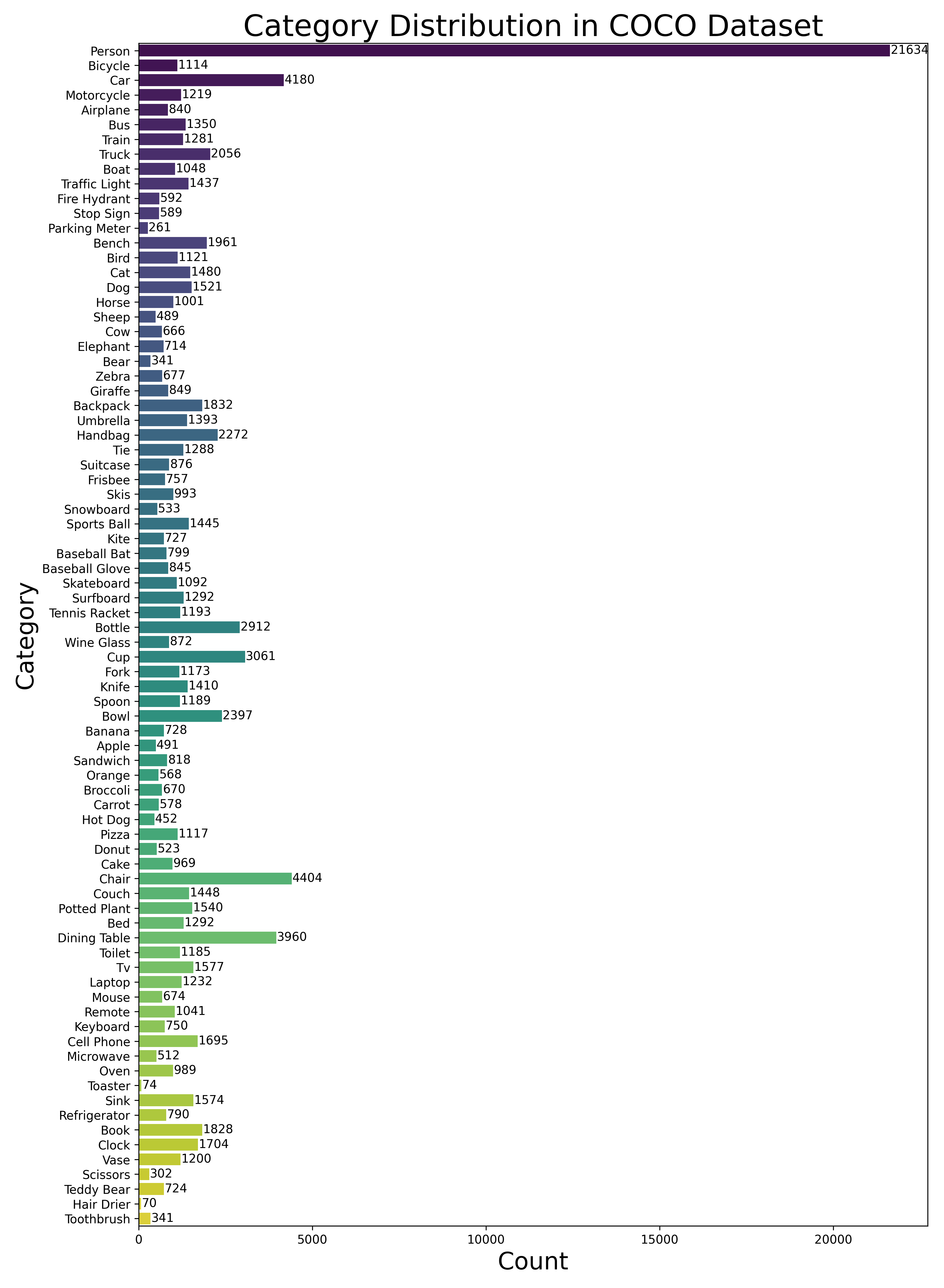
Then plot the distribution of different categories in the validation dataset (2014) to have a clear overview of the imbalancing in the dataset. Feel free to change the dataType to others inculding train2014, train2017, or val2017.

# Initialize the COCO api for instance annotations
coco=COCO(annFile)

# Load the categories in a variable
catIDs = coco.getCatIds()
cats = coco.loadCats(catIDs)

# Get category names
category_names = [cat['name'].title() for cat in cats]

# Get category counts
category_counts = [coco.getImgIds(catIds=[cat['id']]) for cat in cats]
category_counts = [len(img_ids) for img_ids in category_counts]


# Create a color palette for the plot
colors = sns.color_palette('viridis', len(category_names))

# Create a horizontal bar plot to visualize the category counts
plt.figure(figsize=(11, 15))
sns.barplot(x=category_counts, y=category_names, palette=colors)

# Add value labels to the bars
for i, count in enumerate(category_counts):
    plt.text(count + 20, i, str(count), va='center')
plt.xlabel('Count',fontsize=20)
plt.ylabel('Category',fontsize=20)
plt.title('Category Distribution in COCO Dataset',fontsize=25)
plt.tight_layout()
plt.savefig('coco-cats.png',dpi=300)
plt.show()

The output should be:

loading annotations into memory...
Done (t=5.05s)
creating index...
index created!

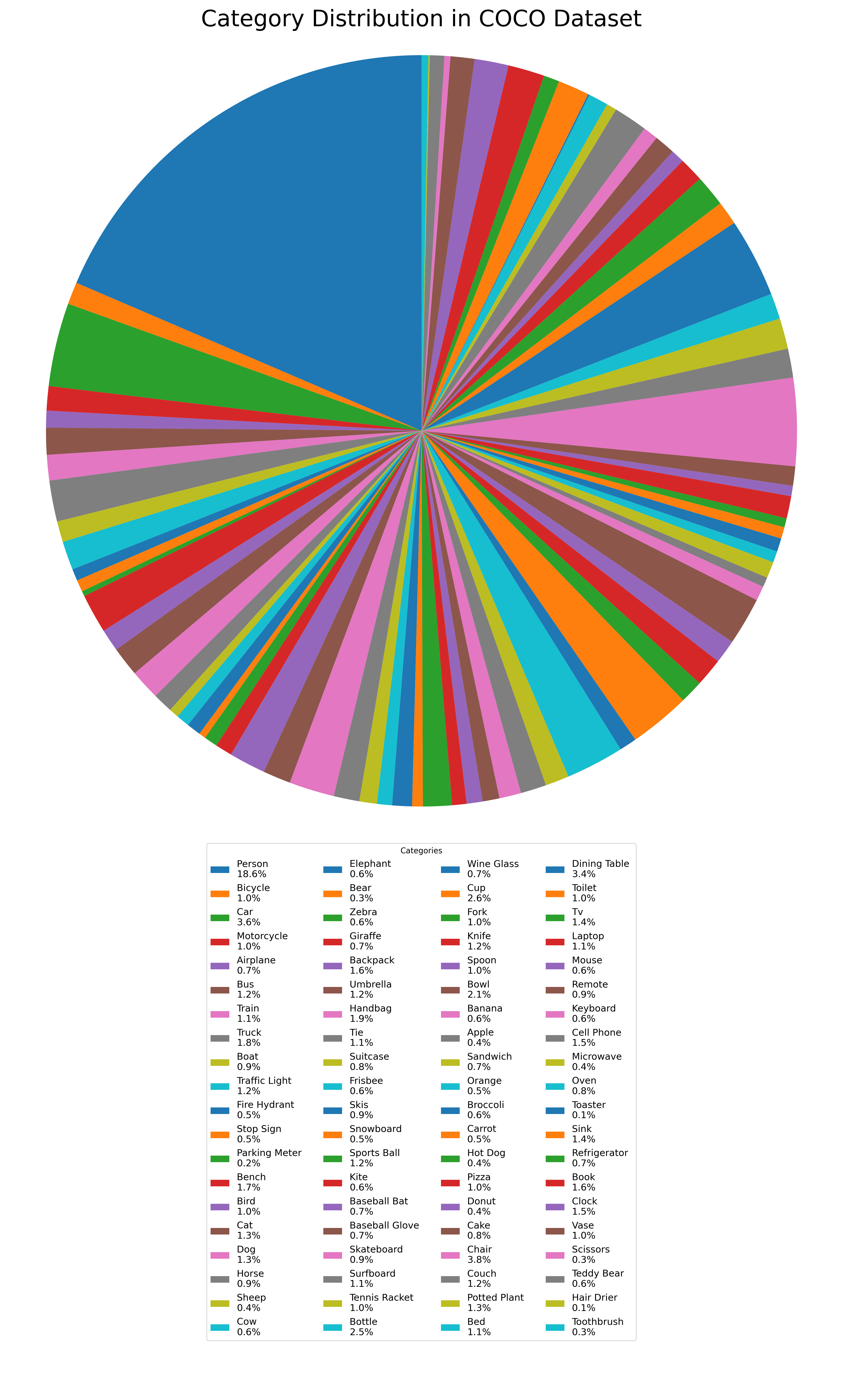
You can use the code below to see the distribution of the categories:

# Calculate percentage for each category
total_count = sum(category_counts)
category_percentages = [(count / total_count) * 100 for count in category_counts]


# Create a pie chart to visualize the category distribution
plt.figure(figsize=(15, 24.9))


# Customize labels properties
labels = [f"{name} " for name, percentage in zip(category_names, category_percentages)]
label_props = {"fontsize": 25, 
               "bbox": {"edgecolor": "white", 
                        "facecolor": "white", 
                        "alpha": 0.7, 
                        "pad": 0.5}
              }

# Add percentage information to labels, and set labeldistance to remove labels from the pie
wedges, _, autotexts = plt.pie(category_counts, 
                              autopct='', 
                              startangle=90, 
                              textprops=label_props, 
                              pctdistance=0.85)

# Create the legend with percentages
legend_labels = [f"{label}\n{category_percentages[i]:.1f}%" for i, label in enumerate(labels)]
plt.legend(wedges, legend_labels, title="Categories", loc="upper center", bbox_to_anchor=(0.5, -0.01), 
           ncol=4, fontsize=12)

plt.axis('equal')
plt.title('Category Distribution in COCO Dataset', fontsize=29)
plt.tight_layout()
plt.savefig('coco-dis.png', dpi=300)
plt.show()

In the following code snippet, we utilize the COCO API to visualize annotations for specific object classes within a dataset. By specifying a list of desired classes, the code filters the dataset to retrieve images containing those classes. A random image is then selected from the filtered images, and its corresponding annotations are loaded. The code proceeds to display the original image along with a bounding box and segmented colors for each annotation. Additionally, a legend is created to associate category names with their assigned colors. This code enables efficient exploration and visualization of specific object classes within a dataset, providing insights into the distribution and characteristics of the selected classes. The resulting visualizations can aid in tasks such as object detection, instance segmentation, and object recognition.

# Define the classes (out of the 80) which you want to see. Others will not be shown.
filterClasses = ['laptop', 'tv', 'cell phone']

# Fetch class IDs only corresponding to the filterClasses
catIds = coco.getCatIds(catNms=filterClasses)

# Get all images containing the above Category IDs
imgIds = coco.getImgIds(catIds=catIds)

# Load a random image from the filtered list
if len(imgIds) > 0:
    image_id = imgIds[np.random.randint(len(imgIds))]  # Select a random image ID
    image_info = coco.loadImgs(image_id)

    if image_info is not None and len(image_info) > 0:
        image_info = image_info[0]
        image_path = imageDir + image_info['file_name']

        # Load the annotations for the image
        annotation_ids = coco.getAnnIds(imgIds=image_id)
        annotations = coco.loadAnns(annotation_ids)

        # Get category names and assign colors for annotations
        category_names = [coco.loadCats(ann['category_id'])[0]['name'].capitalize() for ann in annotations]
        category_colors = list(colors.TABLEAU_COLORS.values())

        # Load the image and plot it
        image = plt.imread(image_path)
        plt.imshow(image)
        plt.axis('off')
        plt.title('Annotations for Image ID: {}'.format(image_id))
        plt.tight_layout()
        plt.savefig('Img.png',dpi=350)
        plt.show()
        
        plt.imshow(image)
        plt.axis('off')

        # Display bounding boxes and segmented colors for each annotation
        for ann, color in zip(annotations, category_colors):
            bbox = ann['bbox']
            segmentation = ann['segmentation']

            # Display bounding box
            rect = patches.Rectangle((bbox[0], bbox[1]), bbox[2], bbox[3], linewidth=1,
                                     edgecolor=color, facecolor='none')
            plt.gca().add_patch(rect)

            # Display segmentation masks with assigned colors
            for seg in segmentation:
                poly = np.array(seg).reshape((len(seg) // 2, 2))
                plt.fill(poly[:, 0], poly[:, 1], color=color, alpha=0.6)

        # Create a legend with category names and colors
        legend_patches = [patches.Patch(color=color, label=name) for color, name in zip(category_colors, category_names)]
        plt.legend(handles=legend_patches, loc="lower center", ncol=4, bbox_to_anchor=(0.5, -0.2), fontsize='small')

        # Show the image with legend
        plt.title('Annotations for Image ID: {}'.format(image_id))
        plt.tight_layout()
        plt.savefig('annImg.png',dpi=350)
        plt.show()
    else:
        print("No image information found for the selected image ID.")
else:
    print("No images found for the desired classes.")

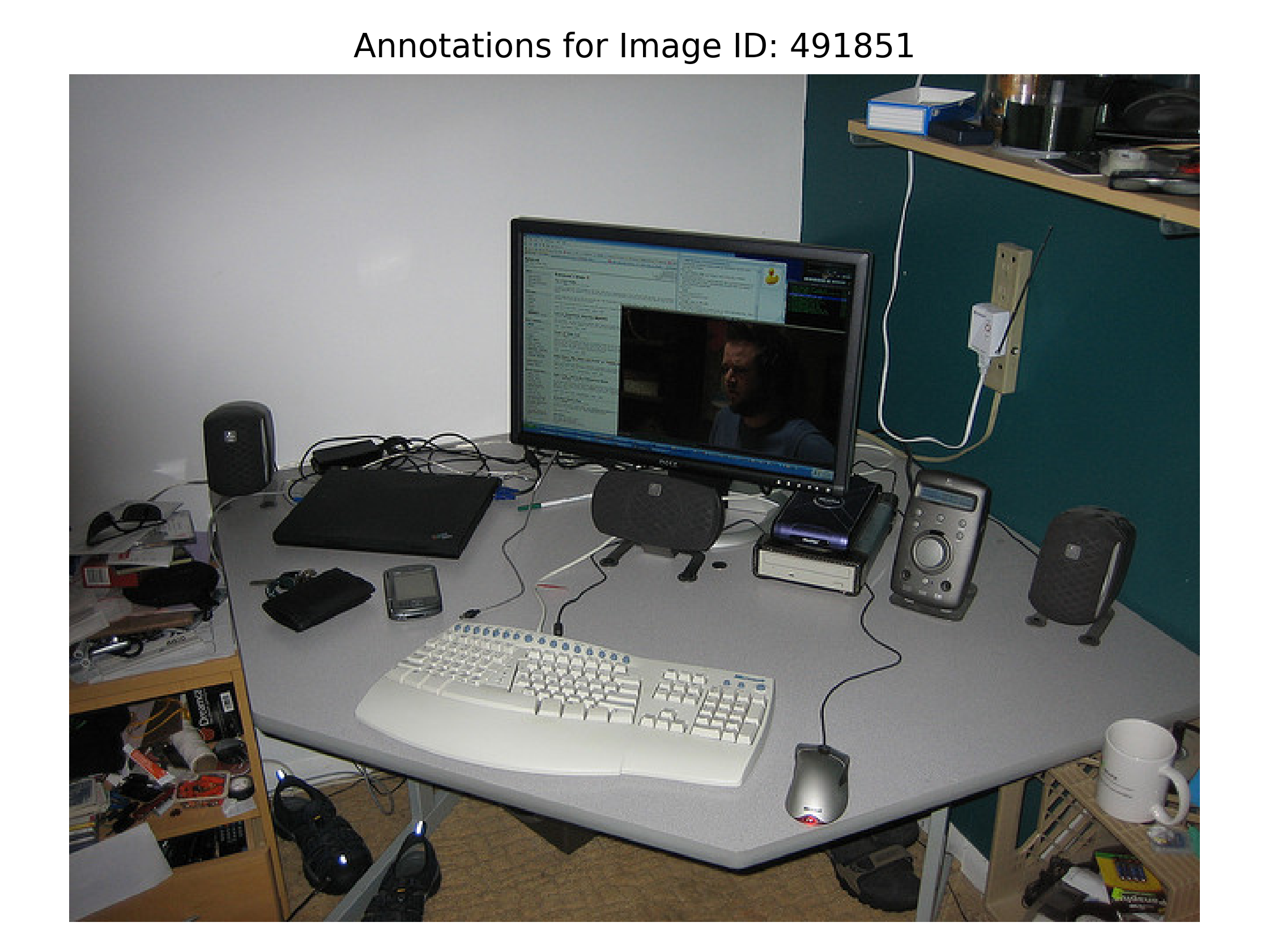
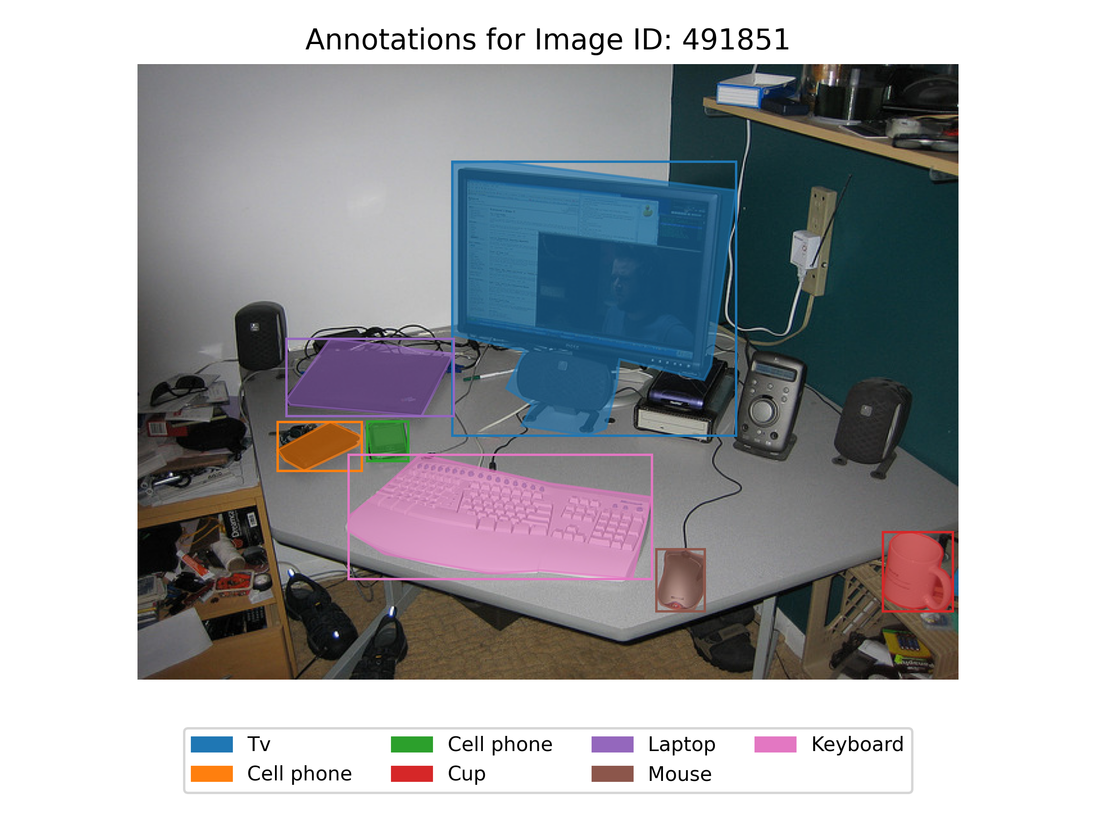
Now we have an overview of the categories in the dataset (don’t worry about the codes, we will delve into each line).

Here’s a detailed explanation of the code and how to use it:

1. First, you need to define the classes of objects that you want to visualize. In the provided code, the filterClasses variable contains a list of desired classes such as ’laptop’, ’tv’, and ‘cell phone’. You can modify this list to include the object classes of your interest.

2. The code uses the COCO API to work with the dataset and annotations. It fetches the category IDs corresponding to the desired classes using coco.getCatIds(catNms=filterClasses). Then, it retrieves the image IDs that contain the specified category IDs with coco.getImgIds(catIds=catIds).

3. If there are images available for the desired classes (if len(imgIds) > 0), the code randomly selects an image ID from the filtered list.

4. The image information is loaded using coco.loadImgs(image_id). If the image information is valid and available, the image path is obtained and stored in image_path.

5. Next, the annotations for the selected image are loaded using coco.getAnnIds(imgIds=image_id) and coco.loadAnns(annotation_ids).

6. The category names and colors are extracted for each annotation. Category names are capitalized, and colors are assigned from the colors.TABLEAU_COLORS dictionary.

7. The original image is loaded and displayed using plt.imshow(image). The plt.axis('off') function is used to turn off the axis labels and ticks.

8. Bounding boxes and segmented colors are displayed for each annotation. Bounding boxes are drawn as rectangles using patches.Rectangle, and segmented colors are filled using the plt.fill function. This process is repeated for each annotation in the image.

9. A legend is created to associate category names with their assigned colors. The legend is displayed using plt.legend and positioned at the lower center of the plot.

10. Finally, the image with annotations and the legend is shown using plt.show().

By following the instructions and modifying the code according to your desired classes, you can visualize annotations for specific object classes in the dataset. This code is useful for gaining insights into the distribution and characteristics of the selected classes, aiding in tasks such as object detection, instance segmentation, and object recognition.

PyCOCO

The PyCOCO library offers helpful function for working with the COCO dataset. Let’s dive deeper into the functions of the COCO class from pycocotools.coco:

First, we import the API by using

from pycocotools.coco import COCO

then you can initialize the COCO API for instance annotations by

dataDir='./'
dataType='val2014'
annFile='{}annotations/instances_{}.json'.format(dataDir,dataType)

coco = COCO(annFile_path)

# Initialize the COCO api for instance annotations
coco=COCO(annFile)

1. loadCats(self, ids=[]): Loads category metadata given their IDs. It returns a list of dictionaries, each representing a category. Each dictionary contains the category id, name, supercategory, and keypoints if available.

# Load categories for the given ids
ids = 1
cats = coco.loadCats(ids=ids)
print(cats)

[{'supercategory': 'person', 'id': 1, 'name': 'person'}]

2. loadImgs(self, ids=[]): Loads image metadata given their IDs. It returns a list of dictionaries, each representing an image. Each dictionary contains the image id, width, height, file name, license, date captured, and COCO URL.

# Load images for the given ids
image_ids = coco.getImgIds()
image_id = image_ids[0]  # Change this line to display a different image
image_info = coco.loadImgs(image_id)
print(image_info)

[{'license': 3,
  'file_name': 'COCO_val2014_000000391895.jpg',
  'coco_url': 'http://images.cocodataset.org/val2014/COCO_val2014_000000391895.jpg',
  'height': 360,
  'width': 640,
  'date_captured': '2013-11-14 11:18:45',
  'flickr_url': 'http://farm9.staticflickr.com/8186/8119368305_4e622c8349_z.jpg',
  'id': 391895}]

3. loadAnns(self, ids=[]): Loads annotations given their IDs. It returns a list of dictionaries, each representing an annotation. Each dictionary contains the annotation id, image id, category id, segmentation, area, bounding box, and whether the annotation is a crowd.

The loadAnns function is used to retrieve annotations for a specific image or a list of annotation IDs. It allows you to access detailed information about each annotation, such as the category of the object, the location of the object in the image, and the shape of the object’s boundary. By using loadAnns, you can obtain a list of annotation objects that contain all the relevant details about the annotations. This function is flexible, allowing you to retrieve annotations for a specific image or fetch annotations based on their unique IDs. It provides a convenient way to access and analyze annotations for various purposes.

# Load annotations for the given ids
annotation_ids = coco.getAnnIds(imgIds=image_id)
annotations = coco.loadAnns(annotation_ids)
print(annotations)

[{'segmentation': [[...]],
  'area': 12190.44565,
  'iscrowd': 0,
  'image_id': 391895,
  'bbox': [359.17, 146.17, 112.45, 213.57],
  'category_id': 4,
  'id': 151091},
 {'segmentation': [[...]],
  'area': 14107.271300000002,
  'iscrowd': 0,
  'image_id': 391895,
  'bbox': [339.88, 22.16, 153.88, 300.73],
  'category_id': 1,
  'id': 202758},
 {'segmentation': [[...]],
  'area': 708.2605500000001,
  'iscrowd': 0,
  'image_id': 391895,
  'bbox': [471.64, 172.82, 35.92, 48.1],
  'category_id': 1,
  'id': 1260346},
 {'segmentation': [[...]],
  'area': 626.9852500000001,
  'iscrowd': 0,
  'image_id': 391895,
  'bbox': [486.01, 183.31, 30.63, 34.98],
  'category_id': 2,
  'id': 1766676}]

4. getCatIds(self, catNms=[], supNms=[], catIds=[]): Gets IDs of categories that satisfy given filter conditions. It can filter by category names, supercategory names, and category IDs.

# Get category ids that satisfy the given filter conditions
filterClasses = ['laptop', 'tv', 'cell phone']
# Fetch class IDs only corresponding to the filterClasses
catIds = coco.getCatIds(catNms=filterClasses)
print(catIds)

[72, 73, 77]

5. getImgIds(self, imgIds=[], catIds=[]): This method gets IDs of images that satisfy given filter conditions. It can filter by image IDs and category IDs.

catID = 15
print(coco.loadCats(ids=catID))

# Get image ids that satisfy the given filter conditions
imgId = coco.getImgIds(catIds=[catID])[0]
print(imgId)

[{'supercategory': 'outdoor', 'id': 15, 'name': 'bench'}]
262148

6. getAnnIds(self, imgIds=[], catIds=[], areaRng=[], iscrowd=None): This method gets IDs of annotations that satisfy given filter conditions. It can filter by image IDs, category IDs, area range, and whether the annotation is a crowd.

# Get annotaions IDs
ann_ids = coco.getAnnIds(imgIds=[imgId], iscrowd=None)
print(ann_ids)

[247584, 576412, 642663, 1209372, 1251030, 1272930, 1277823, 1303789, 1307874, 1312222, 1312550, 1321181, 1324108, 1331011, 1332687, 1371763, 1372845, 1422576, 1837952, 1962686, 2007683, 2061640, 900100262148]

7. loadRes(self, resFile): This method loads results from a file and creates a result API. The results file should be in the COCO result format.

# Load results from a file and create a result API
cocoRes = coco.loadRes(resFile)

8. showAnns(self, anns, draw_bbox=True): This method displays the specified annotations. It can optionally draw the bounding box.

The showAnns function is designed to visualize the annotations on an image. It takes a list of annotation objects and the corresponding image as input. This function overlays the annotations on top of the image, making it easier to understand and interpret the annotations visually. The annotations are typically represented by bounding boxes, which are rectangles that enclose the objects, or segmentation masks, which are pixel-level masks that outline the shape of the objects. By using showAnns, you can see the annotations directly on the image, allowing you to assess the spatial distribution of objects, observe their characteristics, and gain insights into the dataset.

Together, loadAnns and showAnns provide a powerful combination for working with annotations in the COCO dataset. With loadAnns, you can access detailed information about individual annotations, enabling tasks such as object recognition, instance segmentation, or statistical analysis. Then, with showAnns, you can visualize the annotations on the image, helping you to understand and evaluate the dataset visually. These functions are essential for computer vision researchers and practitioners, as they facilitate the exploration, analysis, and interpretation of annotations in the COCO dataset.

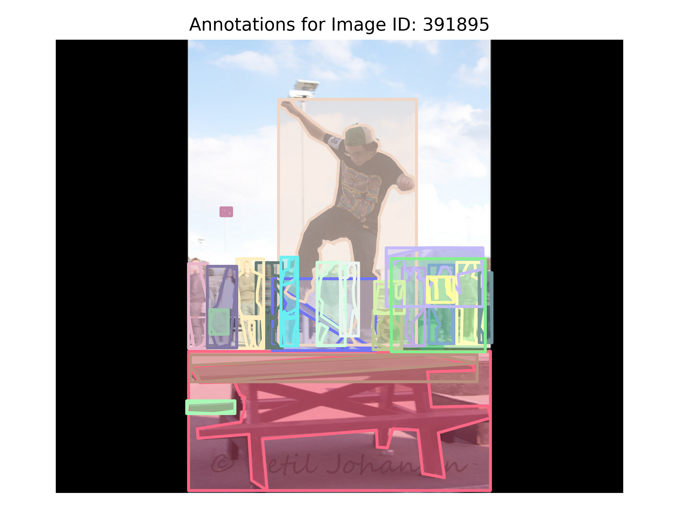
print(f"Annotations for Image ID {imgId}:")
anns = coco.loadAnns(ann_ids)

image_path = coco.loadImgs(imgId)[0]['file_name']
print(image_path)
image = plt.imread(imageDir + image_path)
plt.imshow(image)

# Display the specified annotations
coco.showAnns(anns, draw_bbox=True)

plt.axis('off')
plt.title('Annotations for Image ID: {}'.format(image_id))
plt.tight_layout()
plt.show()

Annotations for Image ID 262148:
COCO_val2014_000000262148.jpg

9. loadNumpyAnnotations(self, data): This method converts a numpy array to the COCO annotation format. The numpy array should have the same structure as the COCO annotation format.

# Convert a numpy array to the COCO annotation format
coco.loadNumpyAnnotations(data)

10. download(self, tarDir, imgIds=[]): This method downloads the COCO images from the server. It requires the target directory and optionally the image IDs.

# Download the COCO images from the server
coco.download(tarDir, imgIds)

Each of these methods provides a different functionality to interact with the COCO dataset, from loading annotations, categories, and images, to getting IDs based on certain conditions, to displaying annotations and downloading images. They are designed to make it easier to work with the COCO dataset in Python.

COCO Dataset Format and Annotations

The COCO dataset follows a structured format using JSON (JavaScript Object Notation) files that provide detailed annotations. Understanding the format and annotations of the COCO dataset is essential for researchers and practitioners working in the field of computer vision. Let’s dive into the precise description of the COCO dataset format and its annotations, with in-depth examples:

JSON File Structure

The COCO dataset comprises a single JSON file that organizes the dataset’s information, including images, annotations, categories, and other metadata.

{
  "info": info, 
  "images": [image], 
  "annotations": [annotation], 
  "licenses": [license],
}

info{
  "year": int, 
  "version": str, 
  "description": str, 
  "contributor": str, 
  "url": str, 
  "date_created": datetime,
}

image{
  "id": int, 
  "width": int, 
  "height": int, 
  "file_name": str, 
  "license": int, 
  "flickr_url": str, 
  "coco_url": str, 
  "date_captured": datetime,
}

license{
  "id": int, 
  "name": str, 
  "url": str,
}

The JSON file follows a hierarchical structure with the following main sections:

1. Info: general information about the dataset, including its version, description, contributor details, and release year. For example:

{
  "info": {
    "version": "1.0",
    "description": "COCO 2017 Dataset",
    "contributor": "Microsoft COCO group",
    "year": 2017,
    "url": "https://...",
    "date_created": "2000-01-01T00:00:00+00:00"
  }
}

1. Licenses: lists the licenses under which the dataset is made available. It includes details such as the license name, ID, and URL. For example:

{
  "licenses": [
    {
      "id": 1,
      "name": "Attribution-NonCommercial",
      "url": "http://creativecommons.org/licenses/by-nc/2.0/"
    },
    ...
  ]
}

1. Images: a list of images in the dataset. Each image is represented as a dictionary and includes information such as the image ID, file name, height, width, and the license under which it is released. For example:

{
  "images": [
    {
      "id": 1,
      "file_name": "000000001.jpg",
      "height": 480,
      "width": 640,
      "license": 1,
      "date_captured": "2014-07-20T19:39:26+00:00"
    },
    ...
  ]
}

1. Annotations: provides annotations for objects present in the images. Each annotation is represented as a dictionary and includes information such as the annotation ID, image ID it belongs to, category ID, segmentation mask, bounding box coordinates, and additional attributes depending on the task. For example:

{
  "annotations": [
    {
      "id": 1,
      "image_id": 1,
      "category_id": 18,
      "segmentation": [[...]],
      "bbox": [39, 63, 203, 112],
      "area": 7225,
      "segmentation": [],
      "iscrowd": 0
    },
    ...
  ]
}

1. Categories: defines the object categories present in the dataset. Each category is represented as a dictionary and includes information such as the category ID and name. For example:

{
  "categories": [
    {
      "id": 1,
      "name": "person"
    },
    ...
  ]
}

6. Captions (optional): This section is specific to image captioning tasks and provides human-authored captions for the images. Each caption is represented as a dictionary and includes information such as the image ID and the caption text. For example:

{
  "annotations": [
    {
      "image_id": 1,
      "caption": "A person walking on a sandy beach."
    },
    ...
  ]
}

Annotation Details

One of the key strengths of the COCO dataset is its rich and detailed annotations. Each image in the dataset is annotated with pixel-level segmentation masks, bounding box coordinates, and category labels which provide precise spatial information about the objects present in the images, enabling tasks such as object detection and instance segmentation.

Moreover, the dataset also includes dense keypoint annotations for human poses, making it suitable for pose estimation and human-centric tasks. The combination of these detailed annotations allows for fine-grained analysis and evaluation of computer vision algorithms.

The annotations in the COCO dataset offer precise spatial information about objects present in the images. The following information is included in the annotations:

• Annotation ID: A unique identifier for each annotation, which helps establish connections between images and their corresponding annotations.

• Image ID: The ID of the image to which the annotation belongs, allowing easy retrieval and association of annotations with their respective images.

• Category ID: The ID of the object category to which the annotation corresponds. It links the annotation to the predefined category defined in the dataset.

• Bounding Box: The coordinates of the bounding box that tightly encloses the object of interest. The bounding box is represented as [x, y, width, height], where (x, y) represents the top-left corner of the bounding box. For example, if the bounding box coordinates are [39, 63, 203, 112], it means the top-left corner of the bounding box is located at (39, 63), and its width and height are 203 and 112 pixels, respectively.

• Segmentation Mask: For instance segmentation tasks, the annotation includes a binary mask that represents the object’s pixel-level segmentation. The mask is a 2D binary array of the same height and width as the image, where pixels belonging to the object are marked as 1, and pixels outside the object are marked as 0. The segmentation mask helps precisely delineate the boundaries of the object. For example, the “segmentation” field in the annotation can contain a list of polygonal coordinates that form the object’s outline.

• Keypoints (optional): For tasks like human pose estimation, the annotation may include keypoint locations representing specific body parts. Each keypoint consists of an (x, y) coordinate and an associated visibility flag. The visibility flag indicates whether the keypoint is visible or occluded in the image. For example, a keypoint annotation might include the coordinates and visibility of body joints like the head, shoulders, elbows, and knees.