Deep Neural Network Implementation Using PyTorch

Introduction
🚀 Dive into the Exciting World of Deep Neural Networks with PyTorch! 🤖🔥
Hey there, fellow tech enthusiast! 🤓 Ever felt like PyTorch is a bit of a puzzle, unlike its more user-friendly counterparts? Well, fret not, because we’re here to spice up your deep learning journey! 🎉
⚡ Introducing the “PyTorch Deep Dive” Series ⚡
Buckle up, because we’re taking you on a whirlwind adventure through the realm of implementing Deep Neural Networks using PyTorch. 🌟 Whether you’re a fresh-faced researcher venturing into the deep learning domain or a pro switching up your frameworks, this series has your back!
📚 It’s Not Your Typical Tutorial 📚
Before we get all technical, let’s set the stage. We’re not going to baby you through PyTorch basics. This isn’t your run-of-the-mill PyTorch tutorial; this is where we show you how to wield the power of PyTorch to craft magnificent Deep Neural Networks. So, if you’ve got your basics down with libraries like NumPy and Matplotlib, you’re golden!
🧠 Deep Dive, Literally 🧠
Hold up! This isn’t Deep Learning 101 either. We’re diving straight into the meaty part – building the real deal! So if you’re nodding your head to terms like Neural Networks and the magic of backpropagation, you’re all set to sail.
🌈 Practical Deep Learning FTW 🌈
Picture this: in our first tutorial, we’re going hands-on with a super simple deep neural network example using PyTorch. 🚀 Trust us, learning through examples is the secret sauce! 🍔🍟 After all, who doesn’t love breaking down complex problems with relatable examples?
🎮 Tutorial Level 1: PyTorch Essentials 🎮
Ready, steady, go! 🏁 We’re kicking things off by giving you the lowdown on PyTorch – why you should use it, what makes it tick, and why it’s your trusty sidekick for the deep learning journey. Then, brace yourself for some action! We’re jumping into a fun classification task. Think of it as a sneak peek into the PyTorch universe: how models are born, trained, and put to the test.
Feeling a bit overwhelmed? No worries at all! Everyone starts somewhere, and this is your starting line. With a sprinkle of patience, a dash of trial and error, and a dollop of dedication, you’ll be whizzing through this in no time.
🚀 Elevate Your Neural Network Game 🚀
Here’s the deal: we’re covering the nitty-gritty, from foundational concepts to crafting your network architecture. By the end of this tutorial, you’ll be waving your PyTorch wand to create powerful deep learning models. 🪄✨
Ready to embark on this journey? We thought so! Head over to the Google Colab notebook at the link below and let’s dive into the world of PyTorch-powered Deep Neural Networks together:
Let’s make those neurons dance and those models shine! 🕺💃💻
Table of Contents
0. What’s the Hype about PyTorch?
PyTorch, the brainchild of the whizzes at Facebook’s AI Research lab (FAIR), is THE open-source framework empowering deep learning daredevils like you. 🎩✨ Whether you’re a research maestro or a coding ninja, PyTorch is your trusty sidekick for crafting and taming deep neural networks that conquer complexity like champs.
0.1 The “Why-Is-PyTorch-Awesome” Showdown
Hold onto your code hats, because PyTorch packs a punch like no other! Here are the dazzling stars that set PyTorch on the red carpet of deep learning fame:
Python Power-Up: PyTorch speaks fluent Python and cozies up with its libraries, making it the ultimate wingman for your Python-powered projects. 🐍📚
Facebook’s Fav: You know it’s a superstar when even Facebook themselves use it for their deep learning endeavors. 📸👑
User-Friendly Vibes: PyTorch brings the party with an API so intuitive, even your pet parrot could grasp it. 🦜💃
Graphs on the Fly: Ever seen a graph build itself while the code dances? PyTorch’s dynamic computational graphs are the coolest party trick in town. 🕺📊
Speed Racer: PyTorch zips through computations faster than a caffeinated cheetah, giving you a turbo-charged coding experience. ⚡🐆
GPU Awesomeness: With CUDA at its side, PyTorch flexes its muscles on GPUs for lightning-fast execution. Cue applause for speed and power! 🚀💥
Community Carnival: Join the PyTorch parade with a bustling community that brings you libraries, tools, and pre-trained models galore! From
torchvisionfor vision quests totransformersfor language escapades, PyTorch’s got you covered. 🎉📚Deploy Delights: PyTorch’s toolkit ensures your models hit the streets with style. Whether you’re sending them to mobile realms or web wonderlands, PyTorch makes sure they’re dressed to impress. 🚀🌐
0.2 The “Code It Like It’s Hot” Vibe
Welcome to the land of Pythonic perfection! 🎉🐍 PyTorch embraces Python’s charm, giving you a playground of simplicity and elegance. It’s a place where you can code complex computations with the grace of a swan in a tutu. 🦢✨
0.3 PyTorch vs. the Universe
Ah, the grand showdown! PyTorch takes on the titans like TensorFlow, Keras, and Caffe. While each has its own fan club, PyTorch stands out like a supernova in a deep learning galaxy:
Dynamic vs. Static: PyTorch’s dynamic graph brings the house down, letting you tweak, twist, and turn your models on the fly. Static graphs, eat your heart out! 💃🎩
Pythonic Powers: PyTorch speaks your language, letting you express complex ideas with Pythonic flair. Say goodbye to tangled code vines! 🐍✨
Debugging Sorcery: PyTorch has your back with debugging tricks up its sleeves. Spot bugs, squash them, and watch your models shine! 🐞🔮
| PyTorch | TensorFlow | Keras | Theano | Lasagne | |
|---|---|---|---|---|---|
| Computational Graph | Dynamic | Static | Static | Symbolic | Symbolic |
| Automatic Differentiation | Yes | Yes | Yes | Yes | Yes |
| GPU Acceleration | Yes | Yes | Yes | Yes | Yes |
| Pythonic API | Yes | Yes | Yes | Partial | No |
| Static Graph Optimization | TorchScript | XLA, Graph Transform Tool (GTT) | N/A | N/A | N/A |
| TensorBoard Integration | Yes | Yes | Yes | No | No |
| Multi-GPU Support | Yes | Yes | Yes | No | No |
| Model Serving and Deployment | TorchServe, TorchScript | TensorFlow Serving, TensorFlow Lite | TensorFlow Serving, TensorFlow Lite | N/A | N/A |
| Parallel and Distributed Training | DistributedDataParallel, DataParallel | tf.distribute.Strategy | tf.distribute.Strategy | No | No |
| Dynamic Neural Networks | Yes | No | No | No | No |
| Mobile and Embedded Deployment | PyTorch Mobile, PyTorch for iOS and Android | TensorFlow Lite | TensorFlow Lite | No | No |
| Quantization Support | Yes | TensorFlow Model Optimization Toolkit | TensorFlow Model Optimization Toolkit | No | No |
| Rich Ecosystem and Community | Yes | Yes | Yes | Limited | Limited |
| Integration with Other Libraries | TorchVision, TorchText, Transformers | TensorFlow Hub, TensorFlow Datasets | TensorFlow Hub, TensorFlow Datasets | Limited | Limited |
| Support and Documentation | Strong | Strong | Strong | Limited | Limited |
Behold the enchanting journey of implementing deep learning in PyTorch, as illustrated below:
- PyTorch Workflow for Deep Learning
- Data Preparation:
- Load and preprocess the dataset:
- Load data from files or libraries.
- Handle missing values and outliers.
- Normalize or scale features if necessary.
- Convert categorical variables to numerical representations.
- Split the dataset:
- Divide data into training, validation, and test sets.
- Shuffle the data to ensure randomness.
- Determine appropriate ratios for each set.
- Load and preprocess the dataset:
- Model Definition:
- Choose a neural network architecture:
- Decide on the type of neural network (e.g., feedforward, convolutional, recurrent).
- Determine the number of layers and units per layer.
- Choose activation functions for hidden layers.
- Define the model’s architecture using PyTorch’s nn.Module:
- Create a custom class inheriting from nn.Module.
- Define layers and operations in the init method.
- Implement the forward pass in the forward method.
- Choose a neural network architecture:
- Loss Function and Optimizer:
- Select a loss function for the task
- Choose an optimizer
- Define learning rate and other hyperparameters.
- Training Loop:
- Iterate over training dataset in batches:
- Divide data into batches for efficient computation.
- Use DataLoader for automatic batching and shuffling.
- Forward pass:
- Pass a batch through the model to obtain predictions.
- Calculate loss:
- Compare predictions to actual target values.
- Compute the loss using the selected loss function.
- Backward pass:
- Calculate gradients using automatic differentiation.
- Backpropagate gradients through the network.
- Update model parameters:
- Use the optimizer to update weights based on gradients.
- Iterate over training dataset in batches:
- Validation:
- Iterate over validation dataset in batches:
- Similar to the training loop but with validation data.
- Calculate validation loss and any desired metrics.
- Evaluate the model’s performance on unseen data.
- Iterate over validation dataset in batches:
- Early Stopping (optional):
- Monitor validation loss during training:
- Track validation loss throughout epochs.
- Compare current loss to previous values.
- Stop if validation loss plateaus or increases:
- Implement a stopping criterion to prevent overfitting.
- Restore the model to the best-performing state.
- Monitor validation loss during training:
- Testing:
- Iterate over test dataset in batches:
- Similar to validation and training loops.
- Calculate test loss and relevant metrics.
- Assess the final model’s performance on unseen data.
- Iterate over test dataset in batches:
- Visualization and Analysis (optional):
- Plot training and validation curves:
- Create graphs of loss and metrics over epochs.
- Visualize model predictions on sample data:
- Display model predictions alongside actual data.
- Gain insights into how the model behaves.
- Plot training and validation curves:
- Save the model.
- Data Preparation:
- PyTorch Workflow for Deep Learning
  - Data Preparation:
      - Load and preprocess the dataset:
          - Load data from files or libraries.
          - Handle missing values and outliers.
          - Normalize or scale features if necessary.
          - Convert categorical variables to numerical representations.
      - Split the dataset:
          - Divide data into training, validation, and test sets.
          - Shuffle the data to ensure randomness.
          - Determine appropriate ratios for each set.
  - Model Definition:
      - Choose a neural network architecture:
          - Decide on the type of neural network (e.g., feedforward, convolutional, recurrent).
          - Determine the number of layers and units per layer.
          - Choose activation functions for hidden layers.
      - Define the model's architecture using PyTorch's nn.Module:
          - Create a custom class inheriting from nn.Module.
          - Define layers and operations in the __init__ method.
          - Implement the forward pass in the forward method.
  - Loss Function and Optimizer:
      - Select a loss function for the task
      - Choose an optimizer
      - Define learning rate and other hyperparameters.
  - Training Loop:
      - Iterate over training dataset in batches:
          - Divide data into batches for efficient computation.
          - Use DataLoader for automatic batching and shuffling.
      - Forward pass:
          - Pass a batch through the model to obtain predictions.
      - Calculate loss:
          - Compare predictions to actual target values.
          - Compute the loss using the selected loss function.
      - Backward pass:
          - Calculate gradients using automatic differentiation.
          - Backpropagate gradients through the network.
      - Update model parameters:
          - Use the optimizer to update weights based on gradients.
  - Validation:
      - Iterate over validation dataset in batches:
          - Similar to the training loop but with validation data.
          - Calculate validation loss and any desired metrics.
          - Evaluate the model's performance on unseen data.
  - Early Stopping (optional):
      - Monitor validation loss during training:
          - Track validation loss throughout epochs.
          - Compare current loss to previous values.
      - Stop if validation loss plateaus or increases:
          - Implement a stopping criterion to prevent overfitting.
          - Restore the model to the best-performing state.
  - Testing:
      - Iterate over test dataset in batches:
          - Similar to validation and training loops.
          - Calculate test loss and relevant metrics.
          - Assess the final model's performance on unseen data.
  - Visualization and Analysis (optional):
      - Plot training and validation curves:
          - Create graphs of loss and metrics over epochs.
      - Visualize model predictions on sample data:
          - Display model predictions alongside actual data.
          - Gain insights into how the model behaves.
  - Save the model.
1. Prerequisites
Before diving into deep neural network implementation with PyTorch, it is essential to have a basic understanding of the following concepts:
- Python programming language
- Machine learning fundamentals
- Neural networks and their architectures
2. Getting Started with PyTorch
Installation
To install PyTorch, you can use pip or conda. Open a terminal and run the following command:
pip install torch torchvision
Also, you can find the comprehensive tutorial on get started in the official page.
Importing Required Libraries
In your Python script or notebook, import the necessary libraries as follows:
import torch
import torch.nn as nn
import torch.optim as optim
import torchvision.transforms as transforms
from torch.utils.data import DataLoader
Setting up the GPU (Optional)
If you have access to a GPU, PyTorch can leverage its power to accelerate computations. To utilize the GPU, ensure that you have the appropriate NVIDIA drivers installed. You can then enable GPU support in PyTorch by adding the following code:
device = torch.device("cuda" if torch.cuda.is_available() else "cpu")
3. Dataset Preparation
In following, we will explore the intricate process of dataset loading, preprocessing, and train-validation-test splitting. We will focus on the MNIST dataset as an illustrative example. By following these steps, you will gain an in-depth understanding of dataset preparation in the context of deep learning.
Data Loading
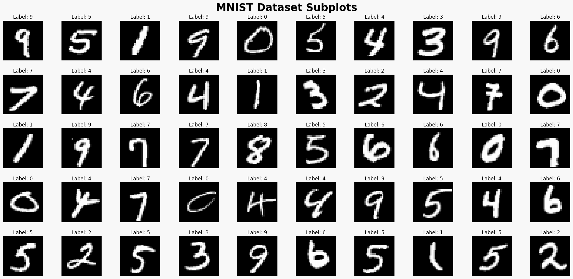
Loading the dataset is the initial step in the data preparation pipeline. PyTorch’s torchvision module provides a range of functions for automatically downloading and loading popular datasets, including MNIST, CIFAR and etc. The MNIST dataset comprises grayscale images of handwritten digits, with each image labeled from 0 to 9.
To load the MNIST dataset using PyTorch, execute the following code:
import torchvision.datasets as datasets

# Define the root directory for dataset storage
data_root = "./data"

# Download and load the MNIST training set
train_set = datasets.MNIST(root=data_root, train=True, download=True)

# Download and load the MNIST test set
test_set = datasets.MNIST(root=data_root, train=False, download=True)
In the above code, we utilize the datasets.MNIST class to download and load the MNIST dataset. The root parameter specifies the directory where the dataset will be stored. By setting train=True, we load the training set, while train=False indicates the test set.
You can visualize the dataset by:
import matplotlib.pyplot as plt
import math

# Define the number of rows and columns for the subplots
num_rows = 5
num_cols = 10

# Calculate the total number of subplots
num_subplots = num_rows * num_cols

# Create a figure and axes for the subplots
fig, axes = plt.subplots(num_rows, num_cols, figsize=(20, 10))


# Iterate over the MNIST dataset and plot the images
for i in range(num_subplots):
    image, label = train_set[i]

    # Convert the image tensor to a numpy array
    image = image.squeeze().numpy()

    # Get the subplot index
    row_idx = i // num_cols
    col_idx = i % num_cols

    # Plot the image in the corresponding subplot
    axes[row_idx, col_idx].imshow(image, cmap='gray')
    axes[row_idx, col_idx].set_title(f'Label: {label}', fontsize=12, pad=5)
    axes[row_idx, col_idx].axis('off')

    # Add a border around each subplot
    axes[row_idx, col_idx].spines['top'].set_visible(True)
    axes[row_idx, col_idx].spines['bottom'].set_visible(True)
    axes[row_idx, col_idx].spines['left'].set_visible(True)
    axes[row_idx, col_idx].spines['right'].set_visible(True)
    axes[row_idx, col_idx].spines['top'].set_color('gray')
    axes[row_idx, col_idx].spines['bottom'].set_color('gray')
    axes[row_idx, col_idx].spines['left'].set_color('gray')
    axes[row_idx, col_idx].spines['right'].set_color('gray')

# Adjust the spacing between subplots
plt.subplots_adjust(wspace=0.2, hspace=0.2)

# Set the overall title and styling
fig.suptitle('MNIST Dataset Subplots', fontsize=25, fontweight='bold', y=0.95)
plt.tight_layout(pad=2)

# Add a background color to the figure
fig.patch.set_facecolor('#F8F8F8')

# Display the subplots
plt.show()
Once the dataset is loaded, it becomes readily available for further processing and model training.
Data Preprocessing
Data preprocessing is a critical step that ensures the dataset is in a suitable format for training a deep neural network. Common preprocessing techniques include normalization, resizing, and data augmentation. PyTorch’s transforms module provides a range of transformation functions to facilitate these preprocessing operations.
Normalization
Normalization is a fundamental preprocessing technique that scales the pixel values to a standardized range. It helps to alleviate the impact of different scales and improves the convergence of the training process. For the MNIST dataset, we can normalize the pixel values to a range of [-1, 1].
To create a preprocessing pipeline specific to the MNIST dataset, use the following code:
import torchvision.transforms as transforms

# Define the transformation pipeline
transform = transforms.Compose([
    transforms.ToTensor(),               # Convert PIL image to tensor
    transforms.Normalize((0.5,), (0.5,)) # Normalize the pixel values to the range [-1, 1]
])

# Apply the transformation pipeline to the training set
train_set.transform = transform

# Apply the transformation pipeline to the test set
test_set.transform = transform
In the code snippet above, we use the ToTensor transformation to convert the PIL images in the dataset to tensors, enabling efficient processing within the deep neural network. Subsequently, the Normalize transformation scales the pixel values by subtracting the mean (0.5) and dividing by the standard deviation (0.5), resulting in a range of [-1, 1].
By applying these transformations, the dataset is effectively preprocessed and ready for training.
Resizing
Resizing is a preprocessing technique commonly employed when input images have varying dimensions. It ensures that all images within the dataset possess consistent dimensions, simplifying subsequent processing steps. However, for the MNIST dataset, the images are already of uniform size (28x28 pixels), so resizing is not necessary in this case.
Data Augmentation
Data augmentation is a powerful technique used to artificially increase the diversity of the training dataset. By applying random transformations to the training images, we introduce additional variations, thereby enhancing the model’s ability to generalize. Common data augmentation techniques include random cropping, flipping, rotation, and scaling.
For the MNIST dataset, data augmentation may not be necessary due to its relatively large size and the inherent variability of the handwritten digits. However, it is worth noting that data augmentation can be beneficial for more complex datasets where additional variations can help improve model performance.
Train-Validation-Test Split
Splitting the dataset into distinct subsets for training, validation, and testing is essential for assessing and fine-tuning the performance of the deep neural network. The train-validation-test split allows us to train the model on one subset, tune hyperparameters on another, and evaluate the final model’s generalization on the independent test set.
PyTorch’s torch.utils.data.random_split utility simplifies this process. We can split the MNIST dataset into training, validation, and test sets using the following code:
from torch.utils.data import random_split

# Define the proportions for the split
train_ratio = 0.7
val_ratio = 0.15
test_ratio = 0.15

# Compute the sizes of each split
train_size = int(len(train_set) * train_ratio)
val_size = int(len(train_set) * val_ratio)
test_size = len(train_set) - train_size - val_size

# Perform the random split
train_set, val_set, test_set = random_split(train_set, [train_size, val_size, test_size])
In the code above, we first import the random_split function from torch.utils.data. We then define the desired proportions for the train, validation, and test sets. The sizes of each split are computed based on these proportions. Finally, we perform the random split on the training set, generating separate datasets for training, validation, and testing.
By splitting the dataset in this manner, we ensure that the model is trained on a sufficiently large training set, validated on a smaller validation set to monitor performance, and tested on an independent test set to evaluate generalization.
4. Model Architecture Design
Designing the architecture of your deep neural network involves selecting the number of layers, their sizes, and the activation functions. Additionally, you need to choose a suitable loss function and optimizer for training the model. Proper selection of hyperparameters is crucial for model performance.
Neural Network Layers
PyTorch provides a variety of layer types, such as fully connected layers (nn.Linear), convolutional layers (nn.Conv2d), and recurrent layers (nn.RNN). These layers can be stacked together to form a deep neural network architecture.
The list of available neural network layers, including but not limited to:
- Convolutional Layers (
nn.Conv1d,nn.Conv2d,nn.Conv3d) - Linear Layers (
nn.Linear) - Recurrent Layers (
nn.RNN,nn.LSTM,nn.GRU) - Dropout Layers (
nn.Dropout,nn.Dropout2d,nn.Dropout3d) - Normalization Layers (
nn.BatchNorm1d,nn.BatchNorm2d,nn.LayerNorm) - Activation Layers (
nn.ReLU,nn.Sigmoid,nn.Tanh,nn.LeakyReLU) - Pooling Layers (
nn.MaxPool1d,nn.MaxPool2d,nn.AvgPool1d,nn.AvgPool2d) - Embedding Layers (
nn.Embedding)
Activation Functions
Activation functions introduce non-linearity to the model. PyTorch offers a wide range of activation functions, including ReLU (nn.ReLU), sigmoid (nn.Sigmoid), and tanh (nn.Tanh).
Here is a list of available activation functions in PyTorch:
- ReLU:
nn.ReLU - Leaky ReLU:
nn.LeakyReLU - PReLU:
nn.PReLU - ELU:
nn.ELU - SELU:
nn.SELU - GELU:
nn.GELU - Sigmoid:
nn.Sigmoid - Tanh:
nn.Tanh - Softmax:
nn.Softmax - LogSoftmax:
nn.LogSoftmax
Loss Functions
The choice of a loss function depends on the task you are trying to solve. PyTorch provides various loss functions, such as mean squared error (nn.MSELoss), cross-entropy loss (nn.CrossEntropyLoss), and binary cross-entropy loss (nn.BCELoss).
Here is a list of available loss functions in PyTorch:
- BCELoss:
nn.BCELoss - BCEWithLogitsLoss:
nn.BCEWithLogitsLoss - CrossEntropyLoss:
nn.CrossEntropyLoss - CTCLoss:
nn.CTCLoss - HingeEmbeddingLoss:
nn.HingeEmbeddingLoss - KLDivLoss:
nn.KLDivLoss - L1Loss:
nn.L1Loss - MarginRankingLoss:
nn.MarginRankingLoss - MSELoss:
nn.MSELoss - MultiLabelMarginLoss:
nn.MultiLabelMarginLoss - MultiLabelSoftMarginLoss:
nn.MultiLabelSoftMarginLoss - MultiMarginLoss:
nn.MultiMarginLoss - NLLLoss:
nn.NLLLoss - PoissonNLLLoss:
nn.PoissonNLLLoss - SmoothL1Loss:
nn.SmoothL1Loss - SoftMarginLoss:
nn.SoftMarginLoss - TripletMarginLoss:
nn.TripletMarginLoss
Optimizers
Optimizers are responsible for updating the model’s parameters based on the computed gradients during training. PyTorch includes popular optimizers like stochastic gradient descent (optim.SGD), Adam (optim.Adam), and RMSprop (optim.RMSprop).
Here is a list of available optimizers in PyTorch:
- SGD:
torch.optim.SGD - Adam:
torch.optim.Adam - RMSprop:
torch.optim.RMSprop - Adagrad:
torch.optim.Adagrad - Adadelta:
torch.optim.Adadelta - AdamW:
torch.optim.AdamW - SparseAdam:
torch.optim.SparseAdam - ASGD:
torch.optim.ASGD - LBFGS:
torch.optim.LBFGS - Rprop:
torch.optim.Rprop
Hyperparameters
Hyperparameters define the configuration of your model and training process. Examples include the learning rate, batch size, number of epochs, regularization strength, and more. Proper tuning of hyperparameters significantly impacts the model’s performance.
5. Building the Deep Neural Network Model
To build and train a deep learning model in PyTorch follow the steps outlined below:
Step 1: Define the Model Architecture
- Start by defining the architecture of your deep learning model. Create a subclass of the
torch.nn.Moduleclass and implement the model’s structure in the__init__method and the forward pass in theforwardmethod. Specify the layers, activation functions, and any other relevant components of your model.
Step 2: Instantiate the Model
- Once the model class is defined, create an instance of the model by instantiating the class with the appropriate parameters. This includes specifying the input size, hidden layer size, and number of output classes.
Step 3: Define the Loss Function
- To train the model, define a loss function that measures the difference between the predicted output and the true labels. Choose an appropriate loss function based on the problem at hand.
Step 4: Define the Optimizer
- Select an optimizer that will update the model’s parameters based on the computed gradients during training. Set the learning rate and other relevant parameters for the optimizer.
Step 5: Train the Model
- Start the training process by iterating over the training dataset in multiple epochs. In each epoch, perform the following steps:
- Iterate over the mini-batches of data (batch size) from the training dataset.
- Perform a forward pass, feeding the input data through the model to obtain predictions.
- Calculate the loss by comparing the predictions with the true labels using the defined loss function.
- Perform a backward pass to compute the gradients of the loss with respect to the model’s parameters.
- Use the optimizer to update the model’s parameters based on the gradients.
- Optionally, track and log the training loss or any other relevant metrics.
Step 6: Evaluate the Model
- After training, evaluate the model’s performance on unseen data to assess its generalization ability. Iterate over the validation or test dataset and calculate relevant metrics, such as accuracy, to measure the model’s performance.
Step 7: Save and Load the Model (Optional)
- If desired, save the trained model to disk for future use or deployment. Use the
torch.save()function to save the model’s state dictionary. Later, load the saved model usingtorch.load()to create an instance of the model and load the saved state.
Throughout the process, ensure that the data is appropriately preprocessed, such as scaling, normalizing, or applying any necessary transformations, to ensure compatibility with the model.
By following these steps, you can build and train a deep learning model in PyTorch. Each step contributes to the overall process of model development, training, evaluation, and potentially saving or loading the model for later use.
When comparing the steps involved in building and training a deep learning model in PyTorch and Keras, both frameworks offer distinct advantages and considerations.
PyTorch:
Flexibility and Control: PyTorch provides a low-level and flexible approach to model development, allowing fine-grained control over the architecture. Its dynamic computational graph enables dynamic network structures and control flow, making it ideal for advanced research and experimentation.
Python Integration: PyTorch seamlessly integrates with the Python ecosystem, leveraging popular libraries like NumPy and SciPy. This integration facilitates efficient data processing, scientific computing, and visualization, empowering researchers with a wide range of tools.
Rich Ecosystem: PyTorch benefits from an active community, resulting in a rich ecosystem of libraries, tools, and pre-trained models. This vibrant community ensures a steady influx of advancements and resources that can be readily utilized.
Keras:
User-Friendly Interface: Keras offers a high-level API built on top of TensorFlow, providing a simplified and intuitive interface. Its design philosophy prioritizes simplicity and ease of use, making it highly accessible for beginners and enabling rapid model iteration.
Quick Prototyping: Keras abstracts away low-level details, allowing for rapid prototyping and easy experimentation. It provides pre-defined models and modules for common deep learning tasks, facilitating quick implementation and practical applications.
In summary, PyTorch’s flexibility and Pythonic approach make it an excellent choice for advanced research and customization, while Keras’s simplicity and abstraction make it preferable for practical applications and rapid prototyping. The choice between the two frameworks depends on the project requirements and the desired trade-off between flexibility and ease of use.
In following, we will delve into how to build and train model using PyTorch.
Defining the Model Class
In the process of building a deep learning model, defining the model class is a fundamental step. This involves creating a class that inherits from the nn.Module base class provided by PyTorch. The model class serves as a blueprint for the architecture of the neural network and encapsulates the layers and the forward propagation logic.
To define the model class, you need to perform the following steps:
Create a class that inherits from
nn.Module, such asNeuralNetwork(nn.Module).- By inheriting from
nn.Module, you can leverage the functionalities and features provided by PyTorch for model construction and training.
- By inheriting from
Define the architecture of the neural network within the
__init__method.def __init__(self, ... ): In the__init__method, you specify the layers and their configurations. This is where you instantiate and define the individual layers of your network. You can considerinput_size, hidden_size, output_sizeto configure the model.- For example, you can use
nn.Linearto create fully connected layers, specifying the input size, output size, and other relevant parameters.super(NeuralNetwork, self).__init__()can be used to initialize the parent class (nn.Module).In Python, when a class inherits from another class, it is important to call the constructor of the parent class to properly initialize its attributes and functionalities. By using
super(NeuralNetwork, self).__init__(), we explicitly call the constructor of thenn.Moduleclass, which is the parent class of our custom model class (NeuralNetwork). This ensures that the necessary initialization steps defined in the parent class are executed before any additional initialization specific to the child class.
Implement the forward propagation logic in the
forwardmethod.- The
forwardmethod defines how the input flows through the network and produces the output. - You apply the necessary activation functions and combine the layers to form the desired network architecture.
- Ensure that the forward pass is defined sequentially, specifying the sequence of operations that transform the input into the output.
- The
Here’s an example of a simple fully connected neural network class:
# Defines a custom model class called NeuralNetwork that inherits from nn.Module. This class will represent our deep learning model.
class NeuralNetwork(nn.Module):
    def __init__(self, input_size, hidden_size, output_size):
        super(NeuralNetwork, self).__init__()  # Initialize the parent class (nn.Module)
        self.fc1 = nn.Linear(input_size, hidden_size)  # Create the first fully connected layer
        self.fc2 = nn.Linear(hidden_size, output_size)  # Create the second fully connected layer
        self.relu = nn.ReLU()  # Initialize the ReLU activation function
        self.dropout = nn.Dropout(0.5)  # Initialize the dropout layer with a dropout probability of 0.5
        self.batchnorm1 = nn.BatchNorm1d(hidden_size)  # Initialize the batch normalization layer for the first layer
        self.batchnorm2 = nn.BatchNorm1d(output_size)  # Initialize the batch normalization layer for the second layer

        # Weight initialization
        nn.init.xavier_uniform_(self.fc1.weight)  # Initialize the weights of the first fully connected layer using the Xavier uniform distribution
        nn.init.xavier_uniform_(self.fc2.weight)  # Initialize the weights of the second fully connected layer using the Xavier uniform distribution

    def forward(self, x):
        x = x.view(x.size(0), -1)  # Reshape the input tensor to a 2D tensor
        x = self.fc1(x)  # Pass the input through the first fully connected layer
        x = self.batchnorm1(x)  # Apply batch normalization to the output of the first layer
        x = self.relu(x)  # Apply the ReLU activation function to the output of the first layer
        x = self.dropout(x)  # Apply dropout to the output of the first layer
        x = self.fc2(x)  # Pass the output through the second fully connected layer
        x = self.batchnorm2(x)  # Apply batch normalization to the output of the second layer
        return x
Initializing the Model
To initialize an instance of the model class, you need to specify the input size, hidden size, and output size. For example:
from torchsummary import summary

input_size = 784  # Number of input features
hidden_size = 128  # Number of hidden units
output_size = 10  # Number of output classes

model = NeuralNetwork(input_size, hidden_size, output_size)  # Create an instance of the NeuralNetwork model

summary(model, (input_size,))  # Print the summary of the model
----------------------------------------------------------------
        Layer (type)               Output Shape         Param #
================================================================
            Linear-1                  [-1, 128]         100,480
       BatchNorm1d-2                  [-1, 128]             256
              ReLU-3                  [-1, 128]               0
           Dropout-4                  [-1, 128]               0
            Linear-5                   [-1, 10]           1,290
       BatchNorm1d-6                   [-1, 10]              20
================================================================
Total params: 102,046
Trainable params: 102,046
Non-trainable params: 0
----------------------------------------------------------------
Input size (MB): 0.00
Forward/backward pass size (MB): 0.00
Params size (MB): 0.39
Estimated Total Size (MB): 0.40
----------------------------------------------------------------
6. Training the Model
Setting up Training Parameters
Before training the model, you need to define the training parameters such as the learning rate, batch size, and number of epochs. You also need to specify the loss function and optimizer.
Defining the Loss Function
Choose an appropriate loss function based on your task. For example, if you are solving a multi-class classification problem, you can use the cross-entropy loss:
criterion = nn.CrossEntropyLoss()
Selecting the Optimizer
Select an optimizer and provide the model parameters to optimize. For example, to use the Adam optimizer:
optimizer = optim.Adam(model.parameters(), lr=0.001)
Define the Number of Epochs
The number of epochs determines how many times the model iterates over the entire training dataset. It is essential to find the right balance: too few epochs may result in underfitting, while too many can lead to overfitting. Researchers employ techniques like early stopping and cross-validation to determine the optimal number of epochs. By fine-tuning this parameter, models can achieve optimal performance without unnecessary computational overhead.
# Define the Number of Epochs
num_epochs = 10
Define the Batch Size
The batch size refers to the number of samples processed in each iteration during training. It plays a crucial role in balancing computational efficiency and model performance. Selecting an appropriate batch size is important to ensure efficient memory utilization and computational speed. A small batch size allows the model to update parameters more frequently but may result in noisy gradients and slower convergence. Conversely, a large batch size reduces noise but may lead to longer training times and potential memory limitations. Researchers often experiment with different batch sizes to find the optimal trade-off between accuracy and computational efficiency for their specific problem. It is important to consider hardware limitations, model complexity, and available computational resources when defining the batch size for training deep learning models.
# Define the Batch Size
batch_size = 32
Creat Dataset Loader
Dataset loaders, such as train_loader and validation_loader, play a crucial role in deep learning. They enable efficient loading and processing of training and validation datasets, respectively. The train_loader iterates through the training data with a specified batch size, allowing for effective model training. The validation_loader evaluates the model’s performance on unseen data. By using dataset loaders, researchers can handle large datasets and ensure effective training and evaluation of deep learning models.
# Create the train_loader
train_loader = torch.utils.data.DataLoader(train_set, batch_size=batch_size, shuffle=True)

# Create the validation_loader
validation_loader = torch.utils.data.DataLoader(val_set, batch_size=batch_size, shuffle=False)
Training the Model
The training loop typically involves iterating over the dataset, performing forward and backward propagation, and updating the model’s parameters. Here’s an example of a basic training loop using PyTorch:
# Initialize empty lists to store metrics
train_losses = []
val_losses = []
accuracies = []

# Proceed with the training loop
for epoch in range(num_epochs):
    model.train()
    running_loss = 0.0
    correct = 0
    total = 0
    for inputs, labels in train_loader:
        inputs = inputs.to(device)  # Move inputs to the GPU if available
        labels = labels.to(device)  # Move labels to the GPU if available

        optimizer.zero_grad()  # Zero the gradients

        outputs = model(inputs)  # Forward pass

        loss = criterion(outputs, labels)  # Compute the loss

        loss.backward()  # Backward pass and optimization
        optimizer.step()

        running_loss += loss.item() * inputs.size(0)  # Update running loss

    train_loss = running_loss / len(train_set)  # Compute average training loss for the epoch

    print(f"Epoch {epoch+1}/{num_epochs}, Training Loss: {train_loss}")  # Print training progress

    # Compute average training loss for the epoch
    train_loss = running_loss / len(train_set)
    train_losses.append(train_loss)

    # Perform validation
    model.eval()
    with torch.no_grad():
        # Perform validation
        validation_loss = 0.0
        correct = 0
        total = 0

        for inputs, labels in validation_loader:
            inputs = inputs.to(device)  # Move inputs to the GPU if available
            labels = labels.to(device)  # Move labels to the GPU if available

            outputs = model(inputs)  # Forward pass

            validation_loss += criterion(outputs, labels).item() * inputs.size(0)  # Compute validation loss

            _, predicted = torch.max(outputs.data, 1)
            total += labels.size(0)
            correct += (predicted == labels).sum().item()

        # Compute average validation loss and accuracy
        val_loss = validation_loss / len(val_set)
        val_losses.append(val_loss)
        accuracy = correct / total * 100
        accuracies.append(accuracy)

        # Print training progress
        print(f"Epoch {epoch+1}/{num_epochs}, Train Loss: {train_loss:.4f}, Val Loss: {val_loss:.4f}, Accuracy: {accuracy:.2f}%")


print("Training complete")
Epoch 1/10, Training Loss: 0.3673658960887364
Epoch 1/10, Train Loss: 0.3674, Val Loss: 0.1725, Accuracy: 96.02%
Epoch 2/10, Training Loss: 0.32074411276408604
Epoch 2/10, Train Loss: 0.3207, Val Loss: 0.1643, Accuracy: 95.98%
Epoch 3/10, Training Loss: 0.2885793504204069
Epoch 3/10, Train Loss: 0.2886, Val Loss: 0.1385, Accuracy: 96.43%
Epoch 4/10, Training Loss: 0.26486541454281126
Epoch 4/10, Train Loss: 0.2649, Val Loss: 0.1290, Accuracy: 96.68%
Epoch 5/10, Training Loss: 0.2510575955793971
Epoch 5/10, Train Loss: 0.2511, Val Loss: 0.1246, Accuracy: 96.89%
Epoch 6/10, Training Loss: 0.23510122887577328
Epoch 6/10, Train Loss: 0.2351, Val Loss: 0.1123, Accuracy: 97.02%
Epoch 7/10, Training Loss: 0.22847037938946768
Epoch 7/10, Train Loss: 0.2285, Val Loss: 0.1097, Accuracy: 97.16%
Epoch 8/10, Training Loss: 0.21747894473870596
Epoch 8/10, Train Loss: 0.2175, Val Loss: 0.1063, Accuracy: 97.22%
Epoch 9/10, Training Loss: 0.2100531817362422
Epoch 9/10, Train Loss: 0.2101, Val Loss: 0.1031, Accuracy: 97.10%
Epoch 10/10, Training Loss: 0.20597965082242375
Epoch 10/10, Train Loss: 0.2060, Val Loss: 0.1013, Accuracy: 97.33%
Training complete
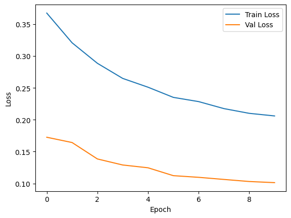
Monitoring Training Progress
During training, it’s helpful to monitor the training loss, validation loss, and accuracy. You can use these metrics to assess the model’s performance and make improvements as necessary. You can also visualize the metrics using libraries like matplotlib or tensorboard.
# Plot training progress
plt.plot(train_losses, label='Train Loss')
plt.plot(val_losses, label='Val Loss')
plt.xlabel('Epoch')
plt.ylabel('Loss')
plt.legend()
plt.show()
7. Evaluating the Model
Testing the Model
Once you have trained the model, you can evaluate its performance on unseen data. Create a separate test data loader and use the trained model to make predictions. Compare the predictions with the ground truth labels to compute metrics such as accuracy, precision, recall, and F1 score.
# Testing the Model
model.eval()  # Set the model to evaluation mode

test_loss = 0.0
correct = 0
total = 0

# Create the test_loader
test_loader = torch.utils.data.DataLoader(test_set, batch_size=batch_size, shuffle=False)

# Disable gradient computation for efficiency
with torch.no_grad():
    for inputs, labels in test_loader:
        inputs = inputs.to(device)  # Move inputs to the GPU if available
        labels = labels.to(device)  # Move labels to the GPU if available

        # Forward pass
        outputs = model(inputs)

        # Compute the loss
        loss = criterion(outputs, labels)
        test_loss += loss.item() * inputs.size(0)

        # Convert output probabilities to predicted class
        _, predicted = torch.max(outputs.data, 1)

        # Update total and correct predictions
        total += labels.size(0)
        correct += (predicted == labels).sum().item()

# Compute average test loss and accuracy
average_loss = test_loss / len(test_set)
accuracy = (correct / total) * 100

print(f"Test Loss: {average_loss:.4f}")
print(f"Accuracy: {accuracy:.2f}%")
Test Loss: 0.1012
Accuracy: 97.13%
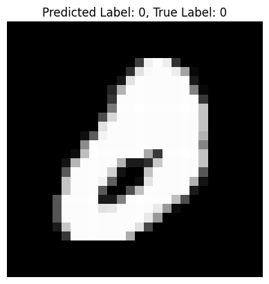
Also, you can test the model by showing an image along with the predicted label, you can select a random sample from the test dataset and visualize the image using matplotlib. Here’s an example of how you can achieve this:
import random
import matplotlib.pyplot as plt

# Set the model to evaluation mode
model.eval()

# Select a random sample from the test dataset
index = random.randint(0, len(test_set) - 1)
image, label = test_set[index]

# Move the image tensor to the same device as the model
image = image.to(device)

# Move the model to the same device as the image
model = model.to(device)

# Forward pass to obtain the predicted label
with torch.no_grad():
    output = model(image.unsqueeze(0))
    _, predicted_label = torch.max(output.data, 1)

# Convert the image tensor to a numpy array
image = image.squeeze().cpu().numpy()

# Display the image and predicted label
plt.imshow(image, cmap='gray')
plt.title(f'Predicted Label: {predicted_label.item()}, True Label: {label}')
plt.axis('off')
plt.show()
Model Evaluation Metrics
The choice of evaluation metrics depends on the specific task you are solving. For classification problems, common metrics include accuracy, precision, recall, and F1 score. For regression tasks, metrics like mean squared error (MSE) or mean absolute error (MAE) are often used.
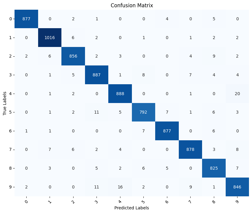
To visualize the performance of a model on the test dataset, you can create a confusion matrix and a classification report. These visualizations provide insights into how well the model is performing for each class in the test dataset.
The following code demonstrates how to evaluate the performance of a deep learning model using the test dataset. It utilizes the sklearn.metrics module to compute the confusion matrix and classification report, which provide insights into the model’s predictions and overall performance.
First, the model is set to evaluation mode using model.eval(). Then, the code iterates through the test loader, disabling gradient computation for efficiency. In each iteration, the model performs a forward pass on the inputs and obtains the predicted class labels. These predicted labels are appended to the predictions list, while the true labels are appended to the true_labels list.
Once all predictions and true labels are collected, the code proceeds to compute the confusion matrix and classification report using the confusion_matrix and classification_report functions from sklearn.metrics. The confusion matrix provides a tabular representation of the model’s predictions versus the true labels, while the classification report offers metrics such as precision, recall, and F1 score for each class.
from sklearn.metrics import confusion_matrix, classification_report

# Get the predictions for the test dataset
model.eval()  # Set the model to evaluation mode
predictions = []
true_labels = []

# Disable gradient computation for efficiency
with torch.no_grad():
    for inputs, labels in test_loader:
        inputs = inputs.to(device)
        labels = labels.to(device)

        # Forward pass
        outputs = model(inputs)

        # Convert output probabilities to predicted class
        _, predicted = torch.max(outputs.data, 1)

        # Append the predicted and true labels
        predictions.extend(predicted.tolist())
        true_labels.extend(labels.tolist())

# Compute the confusion matrix and classification report
cm = confusion_matrix(true_labels, predictions)
report = classification_report(true_labels, predictions)

# Print the confusion matrix and classification report
print("Confusion Matrix:")
print(cm)
print("\nClassification Report:")
print(report)
Confusion Matrix:
[[ 877    0    2    1    0    0    4    0    5    0]
 [   0 1016    6    2    0    1    0    1    2    2]
 [   2    6  856    2    3    0    0    4    9    2]
 [   0    1    5  887    1    8    0    7    4    4]
 [   0    1    2    0  888    0    0    1    0   20]
 [   0    1    2   11    5  792    7    1    6    3]
 [   1    1    0    0    0    7  877    0    6    0]
 [   0    7    6    2    4    0    0  878    3    8]
 [   0    3    0    5    2    6    5    0  825    7]
 [   2    0    0   11   16    2    0    9    1  846]]

Classification Report:
              precision    recall  f1-score   support

           0       0.99      0.99      0.99       889
           1       0.98      0.99      0.98      1030
           2       0.97      0.97      0.97       884
           3       0.96      0.97      0.97       917
           4       0.97      0.97      0.97       912
           5       0.97      0.96      0.96       828
           6       0.98      0.98      0.98       892
           7       0.97      0.97      0.97       908
           8       0.96      0.97      0.96       853
           9       0.95      0.95      0.95       887

    accuracy                           0.97      9000
   macro avg       0.97      0.97      0.97      9000
weighted avg       0.97      0.97      0.97      9000
To create a visually appealing confusion matrix, you can use the heatmap function from the seaborn library. This will allow you to plot the confusion matrix as a color-coded image, making it easier to interpret.
Here’s an example of how to create a beautiful confusion matrix using seaborn:
import seaborn as sns
import matplotlib.pyplot as plt
from sklearn.metrics import confusion_matrix

# Compute the confusion matrix
cm = confusion_matrix(true_labels, predictions)

# Create a figure and axes for the confusion matrix plot
fig, ax = plt.subplots(figsize=(10, 8))

# Create a heatmap of the confusion matrix
sns.heatmap(cm, annot=True, cmap='Blues', fmt='d', cbar=False, ax=ax)

# Set the axis labels and title
ax.set_xlabel('Predicted Labels')
ax.set_ylabel('True Labels')
ax.set_title('Confusion Matrix')

# Customize the tick labels
tick_labels = range(len(cm))
ax.set_xticklabels(tick_labels)
ax.set_yticklabels(tick_labels)

# Rotate the tick labels for better visibility
plt.xticks(rotation=45)
plt.yticks(rotation=0)

# Show the plot
plt.show()
In this code, we first compute the confusion matrix using the confusion_matrix function from scikit-learn. Then, we create a figure and axes for the plot using plt.subplots. We use the sns.heatmap function to create a heatmap of the confusion matrix, with annotations to display the values in each cell. We customize the colormap (cmap) to use the ‘Blues’ color scheme and set fmt='d' to display the cell values as integers.
We set the axis labels and title, and customize the tick labels to match the class labels. Finally, we rotate the tick labels for better visibility and display the plot using plt.show().
This code will produce ab informative visualization of the confusion matrix, allowing you to easily interpret the model’s performance on the test dataset.
8. Improving Model Performance
To improve the performance of your deep neural network model, you can employ various techniques.
Regularization Techniques
Regularization helps prevent overfitting. Techniques like L1 and L2 regularization (weight decay), dropout, and batch normalization can be applied to the model.
Hyperparameter Tuning
Tuning hyperparameters is crucial for achieving optimal performance. You can use techniques like grid search, random search, or more advanced methods like Bayesian optimization to find the best combination of hyperparameters.
Data Augmentation
Data augmentation involves applying transformations to the training data to increase its diversity. Techniques like random cropping, flipping, rotation, and scaling can be used to augment the dataset, thereby improving generalization.
Transfer Learning
Transfer learning allows you to leverage pre-trained models trained on large datasets and adapt them to your specific task. By using pre-trained models as a starting point, you can significantly reduce training time and achieve good performance with limited labeled data.
9. Saving and Loading Models
Saving the Model
You can save the trained model’s parameters to disk for future use or deployment. PyTorch provides the torch.save function to save the model. Here’s an example:
torch.save(model.state_dict(), 'model.pth')
Loading the Model
To load the saved model, create an instance of the model class and load the saved parameters. Here’s an example:
model = NeuralNetwork(input_size, hidden_size, output_size)
model.load_state_dict(torch.load('model.pth'))
model.eval()
10. Conclusion
In this tutorial, we covered the complete process of implementing a deep neural network using PyTorch. We explored data loading and preprocessing, model architecture design, training, evaluation, and techniques for improving model performance. By leveraging PyTorch’s capabilities, you can build and train powerful deep learning models for a wide range of tasks.
11. References
Here are some references that you may find useful for further exploration:
- PyTorch documentation: https://pytorch.org/docs/
- PyTorch tutorials: https://pytorch.org/tutorials/
- Official PyTorch GitHub repository: https://github.com/pytorch/pytorch
Arman Asgharpoor Golroudbari
Machine Learning Engineer
Machine Learning Engineer with 5+ years of experience in LLMs, transformer architectures, computer vision systems, and autonomous robotics.