Comprehensive PyTorch Tutorial: Implementing a Neural Network Class

🎉 Welcome to this tutorial on implementing a Neural Network class using PyTorch! 🎉

In this tutorial, we will focus on building a Neural Network class in PyTorch and go through each step in detail, explaining every part of the Neural Network class, so you can understand the underlying concepts thoroughly.

• Comprehensive PyTorch Tutorial: Implementing a Neural Network Class
  • 1. Introduction to Neural Networks 🧠
    • 1.1 The Neurons - Building Blocks of a Neural Network
    • 1.2 Learning Superpowers 💪
    • 1.3 Building a Neural Network 🛠️
    • 1.4 The Amazing Forward Pass 🏃‍♂️
    • 1.5 Learning from Mistakes 🧠⚡
  • 2. Building Blocks of a Neural Network
    • Input Layer
    • Hidden Layers
    • Output Layer
    • 3. Defining the Neural Network Model Class
    • 3.1 Parts of the Neural Network Model Class
      • 3.1.1 The Constructor Method
      • 3.1.2 The Forward Method
      • 3.1.3 The Input Layer
      • 3.1.4 The Hidden Layers
      • 3.1.5 The Output Layer
    • 3.2 Defining the Neural Network Model Class in Code
      • Explanation:
    • 3.3 Summary
  • 4. Implementing Forward Propagation
  • 5. Backpropagation and Training
  • 6. Adding Activation Functions
  • 7. Customizing Loss Functions
  • 8. Optimizers for Training
  • 9. Putting It All Together: Example Usage
  • 10. Conclusion

Let’s get started!

1. Introduction to Neural Networks 🧠

[Credit: Alex Lenail].

Neural Networks are fascinating and powerful models inspired by the intricate structure of the human brain. They have revolutionized the field of artificial intelligence and are at the core of many modern machine learning advancements. In this introduction, we will delve into the inner workings of Neural Networks, exploring their architecture, learning process, and applications.

1.1 The Neurons - Building Blocks of a Neural Network

At the heart of a Neural Network are artificial neurons, also known as nodes. These neurons are analogous to the neurons in the human brain, and they are responsible for processing and transmitting information. Each neuron takes input from other neurons or external data, processes it using learnable parameters (weights and biases), and then produces an output. These outputs serve as inputs for the neurons in the next layer, creating a cascade of interconnected information flow.

1.2 Learning Superpowers 💪

The learning process in Neural Networks is a marvel of computational intelligence. During training, the network learns from labeled examples to adjust its learnable parameters (weights and biases). This optimization process aims to minimize a predefined loss function that measures the difference between the predicted outputs and the true labels.

To achieve this, the network utilizes a powerful algorithm called backpropagation. During backpropagation, the network’s performance on the training data is evaluated, and the gradients of the loss function with respect to the learnable parameters are calculated. These gradients indicate the direction and magnitude of adjustments needed to minimize the loss. The network then uses optimization algorithms, like stochastic gradient descent (SGD) or Adam, to update the parameters accordingly.

1.3 Building a Neural Network 🛠️

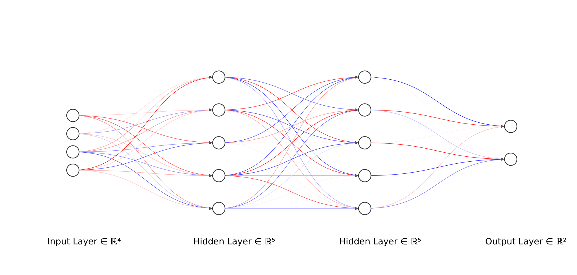
To construct a Neural Network, we first decide on its architecture. This includes determining the number of layers, the number of neurons in each layer, and the connections between them. The first layer is the input layer, which receives the raw input data. The last layer is the output layer, responsible for producing the final predictions or outcomes of the network.

In between the input and output layers, we have one or more hidden layers. These layers are the powerhouse of the network, as they perform the complex computations and feature extraction required for learning intricate patterns in the data. The number of hidden layers and the number of neurons in each layer are hyperparameters that depend on the problem’s complexity and the size of the dataset.

1.4 The Amazing Forward Pass 🏃‍♂️

Once we have our Neural Network architecture set up, it’s time for the forward pass! During the forward pass, data flows through the network from the input layer to the output layer. At each neuron, the input data is multiplied by the corresponding weights, and biases are added to create a weighted sum. This sum is then passed through an activation function, like the popular Rectified Linear Unit (ReLU) or Sigmoid, to introduce non-linearity to the model.

The result of each neuron’s computation becomes the input for the neurons in the next layer. This sequential computation through the layers enables the network to learn increasingly abstract and higher-level representations of the input data.

1.5 Learning from Mistakes 🧠⚡

After the forward pass, the network compares its predictions with the true labels of the training data. The discrepancies between the predicted outputs and the true labels are quantified using a loss function, such as mean squared error or cross-entropy loss. The goal during training is to minimize this loss, effectively reducing the difference between the predicted and true values.

2. Building Blocks of a Neural Network

A basic Neural Network consists of three main components:

Input Layer

The input layer receives the data and passes it to the next layer. The number of neurons in this layer corresponds to the size of the input data.

Hidden Layers

The hidden layers process the input data through a series of transformations. They learn to extract relevant features from the data, enabling the network to make accurate predictions.

Output Layer

The output layer produces the final predictions or outputs of the model. The number of neurons in this layer is determined by the task (e.g., binary classification, multi-class classification, regression).

3. Defining the Neural Network Model Class

In this section, we will thoroughly explore the process of defining the Neural Network Model class in PyTorch. Understanding this fundamental step is crucial for building advanced neural networks for various machine learning tasks. We will discuss each component of the class in detail, explain their significance, and provide illustrative code examples to solidify our understanding.

3.1 Parts of the Neural Network Model Class

3.1.1 The Constructor Method

The constructor method (__init__) is the starting point for building our Neural Network Model class. It is called when an instance of the class is created and sets up the architecture of the neural network. This method allows us to define various parameters, such as the input size, hidden layer sizes, and output size, enabling us to customize the model based on the task at hand. The constructor is vital because it specifies the model’s architecture and provides a way to set hyperparameters and other configurations.

3.1.2 The Forward Method

The forward method is the heart of the Neural Network Model class. It defines how input data flows through the network to produce predictions. During the forward pass, data goes through each layer sequentially, and activation functions are applied to introduce non-linearity. This process allows the neural network to learn complex patterns and relationships from the input data. The forward method is essential for enabling efficient computation and automatic differentiation during backpropagation, which is the key to training the neural network.

3.1.3 The Input Layer

The input layer of the neural network is the initial layer that receives the raw input data and connects it to the first hidden layer. The number of neurons in the input layer is determined by the size of the input data, which, in turn, defines the number of features or input dimensions. Each neuron in the input layer corresponds to one feature of the input data, and these neurons act as entry points to the neural network.

3.1.4 The Hidden Layers

The hidden layers of the neural network are where the real computation and feature extraction occur. Each hidden layer contains multiple neurons (also known as nodes), and these neurons are fully connected to the neurons in the previous and subsequent layers. The hidden layers process the input data through a series of linear transformations followed by activation functions. These activations introduce non-linearity to the model, enabling it to learn complex patterns from the data. The number of hidden layers and the number of neurons in each layer are crucial hyperparameters that significantly impact the model’s performance.

3.1.5 The Output Layer

The output layer of the neural network produces the final predictions or outputs. The number of neurons in the output layer depends on the nature of the task. For example, in binary classification problems, there is usually one neuron for a single output representing the probability of belonging to one class. In multi-class classification problems, there are multiple neurons, each corresponding to a class, and the highest activation value determines the predicted class label. In regression tasks, the output layer might have a single neuron to predict a continuous value.

3.2 Defining the Neural Network Model Class in Code

Now that we have discussed the fundamental components of the Neural Network Model class, let’s proceed with the code implementation. We will define each part of the class and explain its significance along the way.

import torch
import torch.nn as nn
import torch.nn.functional as F

class NeuralNetworkModel(nn.Module):
    def __init__(self, input_size, hidden_sizes, output_size):
        super(NeuralNetworkModel, self).__init__()
        self.input_size = input_size
        self.hidden_sizes = hidden_sizes
        self.output_size = output_size

        # Create the layers for the neural network
        self.input_layer = nn.Linear(self.input_size, self.hidden_sizes[0])
        self.hidden_layers = nn.ModuleList([
            nn.Linear(hidden_sizes[i], hidden_sizes[i + 1]) for i in range(len(hidden_sizes) - 1)
        ])
        self.output_layer = nn.Linear(self.hidden_sizes[-1], self.output_size)

    def forward(self, x):
        # Define the forward pass through the neural network
        x = F.relu(self.input_layer(x))
        for layer in self.hidden_layers:
            x = F.relu(layer(x))
        x = self.output_layer(x)
        return x

Explanation:

1. We start by importing the required libraries: torch, torch.nn, and torch.nn.functional. These libraries contain essential tools for building and training neural networks in PyTorch.

2. We define the NeuralNetworkModel class and inherit from nn.Module, which is the base class for all PyTorch models. By inheriting from nn.Module, our class gains several functionalities, including the ability to hold parameters, manage sub-modules, and perform backpropagation efficiently.

3. In the __init__ method, we specify the constructor of the class. It takes three arguments:

   • input_size: The number of features in the input data, which determines the number of neurons in the input layer.
   • hidden_sizes: A list that specifies the number of neurons in each hidden layer. The length of this list determines the number of hidden layers in the network.
   • output_size: The number of neurons in the output layer, which is determined by the task (e.g., binary classification, multi-class classification, regression).

4. We call the __init__ method of the parent class (nn.Module) using super(NeuralNetworkModel, self).__init__() to properly initialize the nn.Module functionalities.

5. Next, we create the layers for our neural network:

   • self.input_layer: This is the input layer, created using nn.Linear(self.input_size, self.hidden_sizes[0]). It connects the input data to the first hidden layer and performs a linear transformation.
   • self.hidden_layers: This is a list of hidden layers, created using a list comprehension. Each hidden layer is an instance of nn.Linear and is initialized

with the number of neurons specified in the hidden_sizes list.

• self.output_layer: This is the output layer, created using nn.Linear(self.hidden_sizes[-1], self.output_size). It connects the last hidden layer to the output data and performs a linear transformation.

6. In the forward method, we define the forward pass of the neural network. It takes an input x and applies the layers in sequence:

   • x = F.relu(self.input_layer(x)): The input data x passes through the input layer, and the ReLU activation function (F.relu) is applied. ReLU introduces non-linearity to the model, allowing it to learn complex patterns from the data.
   • for layer in self.hidden_layers:: We use a loop to sequentially pass the data through each hidden layer.
   • x = F.relu(layer(x)): At each hidden layer, we apply the ReLU activation function again.
   • x = self.output_layer(x): Finally, the data flows through the output layer to produce the final predictions.

7. The method returns the output x, which contains the predictions made by the neural network.

3.3 Summary

In this extensive section, we have learned how to define the Neural Network Model class in PyTorch comprehensively. We discussed the essential components of the class, such as the constructor method, the forward method, the input layer, the hidden layers, and the output layer.

Understanding the intricacies of defining a neural network class is a critical step in mastering deep learning with PyTorch. By customizing the architecture and layers of the class, you can build powerful and versatile neural network models for various machine learning tasks.

In the next sections, we will delve into backpropagation, optimization, activation functions, loss functions, training loops, and more, further enhancing our knowledge of deep learning with PyTorch.

Keep up the excellent work, and let’s continue our exciting journey into the world of neural networks! 🚀🧠

4. Implementing Forward Propagation

The forward method is the heart of the neural network class. It defines the forward pass, where input data moves through the network to produce predictions.

For our neural network class, the forward pass involves passing the input data through the input layer, applying ReLU activation to the hidden layers, and then passing through the output layer.

5. Backpropagation and Training

To train a neural network, we need to perform backpropagation. It is the process of computing gradients and updating weights and biases to minimize the defined loss function.

We use an optimizer, such as torch.optim.SGD or torch.optim.Adam, to update the parameters of the model during training.

6. Adding Activation Functions

Activation functions introduce non-linearity to the model, allowing it to learn complex patterns from the data. In our neural network class, we use the Rectified Linear Unit (ReLU) activation function for the hidden layers. However, PyTorch provides various activation functions, and you can experiment with them based on your specific problem.

7. Customizing Loss Functions

The choice of loss function depends on the task at hand. For example, for binary classification problems, we often use Binary Cross Entropy Loss, while for multi-class classification, we use Cross Entropy Loss. For regression tasks, Mean Squared Error (MSE) is a common choice. You can customize the loss function in the training process based on your specific needs.

8. Optimizers for Training

PyTorch provides various optimizers like Stochastic Gradient Descent (SGD), Adam, RMSprop, etc. The optimizer updates the model’s parameters during backpropagation to minimize the loss function.

9. Putting It All Together: Example Usage

Now, let’s put all the pieces together and see how to use our custom NeuralNetworkModel class for a specific task.

# Example usage of the NeuralNetworkModel class

# Assuming we have a dataset with 10 input features and want to predict 3 classes
input_size = 10
hidden_sizes = [64, 32]  # Two hidden layers with 64 and 32 neurons, respectively
output_size = 3

# Create an instance of the NeuralNetworkModel class
model = NeuralNetworkModel(input_size, hidden_sizes, output_size)

# Define the loss function and optimizer
criterion = nn.CrossEntropyLoss()
optimizer = torch.optim.SGD(model.parameters(), lr=0.01)

# Training loop
num_epochs = 100
for epoch in range(num_epochs):
    # Forward pass
    outputs = model(input_data)
    loss = criterion(outputs, target_labels)

    # Backward pass and optimization
    optimizer.zero_grad()
    loss.backward()
    optimizer.step()

    # Print the loss at

 certain intervals to monitor training progress
    if (epoch + 1) % 10 == 0:
        print(f"Epoch [{epoch + 1}/{num_epochs}], Loss: {loss.item():.4f}")

# After training, you can use the model for predictions
with torch.no_grad():
    model.eval()
    test_outputs = model(test_input_data)
    predicted_labels = torch.argmax(test_outputs, dim=1)
    print("Predictions:", predicted_labels)

10. Conclusion

Congratulations! You have successfully implemented a comprehensive Neural Network Model class using PyTorch. We covered the fundamental building blocks of neural networks, the steps involved in building the model class, and how to use it for training and prediction.

By understanding this tutorial, you now have a solid foundation to explore and experiment with more complex neural network architectures and tackle various machine learning tasks using PyTorch.

Remember, practice is key to mastering the art of deep learning. Keep experimenting, learning, and building exciting projects. 🚀

Happy coding! 😊🎓