Spacecraft Trajectory Optimization
- Spacecraft Trajectory Optimization
- Introduction
- Prerequisites
- Goals
- Table of Contents
- 1. Problem Formulation
- 2. Mathematical Models in Spacecraft Trajectory Optimization
- Mathematical Models in Spacecraft Trajectory Optimization
- \end{bmatrix} - Classical Orbital Elements - Modified Equinoctial Orbital Elements - 2.2.2 Rendezvous - 2.2.3 Libration points
Spacecraft Trajectory Optimization
Introduction
Spacecraft trajectory optimization plays a pivotal role in the realm of aerospace engineering, enabling the design of efficient and feasible paths for spacecraft to traverse between different points in space while considering a multitude of constraints and objectives. In this post we aimed to delve into advanced techniques and methodologies for spacecraft trajectory optimization.
Space missions demand precise and optimal trajectory planning to achieve desired objectives, such as minimizing fuel consumption, reducing mission duration, reaching specific targets, or avoiding hazardous areas. Additionally, spacecraft dynamics, propulsion systems, and mission constraints impose numerous challenges that necessitate the application of sophisticated optimization methods.
This post will offer a comprehensive exploration of spacecraft trajectory optimization, encompassing both theoretical foundations and practical implementation using Python. By investigating diverse optimization algorithms, formulating optimization problems, and employing visualization techniques, readers will develop the necessary expertise to address intricate trajectory optimization challenges.
To engage in this tutorial effectively, a solid understanding of astrodynamics is presumed, encompassing key concepts such as orbital mechanics, spacecraft dynamics, and orbital transfers. Proficiency in optimization theory and numerical methods is also advantageous. Furthermore, competence in Python programming is essential, as we will utilize prominent scientific libraries like NumPy, SciPy, and matplotlib to realize and evaluate spacecraft trajectory optimization algorithms.
The primary objectives of this tutorial are as follows:
- Attain an encompassing comprehension of spacecraft trajectory optimization, encompassing problem formulation, decision variables, objective functions, and constraints.
- Explore advanced optimization algorithms suitable for spacecraft trajectory optimization, including both direct and indirect methods.
- Implement spacecraft trajectory optimization algorithms utilizing Python, employing numerical techniques and optimization libraries.
- Visualize and analyze optimized trajectories to gain insightful perspectives on spacecraft trajectory performance.
By the conclusion of this tutorial, participants will possess the requisite knowledge and competencies to address intricate spacecraft trajectory optimization problems. They will be proficient in formulating trajectory optimization problems, implementing optimization algorithms in Python, and effectively interpreting and visualizing results. This acquired expertise will empower them to contribute to the design and planning of space missions, enabling the realization of efficient and precise spacecraft trajectories for a broad spectrum of applications, ranging from satellite deployments to interplanetary missions and beyond.
Prerequisites
To make the most of this tutorial, you should have a solid understanding of astrodynamics, optimization theory, and Python programming. Familiarity with numerical methods and scientific computing libraries such as NumPy, SciPy, and matplotlib will be highly beneficial.
Goals
By the end of this tutorial, you will be able to:
- Understand the fundamentals of spacecraft trajectory optimization.
- Formulate trajectory optimization problems with different objectives and constraints.
- Implement advanced optimization algorithms to solve spacecraft trajectory problems.
- Visualize and analyze the optimized trajectories using Python.
Table of Contents
- Spacecraft Trajectory Optimization
- Introduction
- Prerequisites
- Goals
- Table of Contents
- 1. Problem Formulation
- 2. Mathematical Models in Spacecraft Trajectory Optimization
- Mathematical Models in Spacecraft Trajectory Optimization
- \end{bmatrix} - Classical Orbital Elements - Modified Equinoctial Orbital Elements - 2.2.2 Rendezvous - 2.2.3 Libration points
1. Problem Formulation
Spacecraft trajectory optimization is a complex and challenging area of research in astrodynamics. It involves determining an optimal trajectory for a spacecraft while considering specified initial and terminal conditions and minimizing or maximizing a chosen objective. The primary objective often revolves around minimizing propellant usage or maximizing the available mass for non-propellant components. However, other objectives such as minimizing flight time or optimizing the trajectory shape may also be important, depending on the mission requirements.
Spacecraft trajectory optimization poses several inherent complexities. The dynamics governing spacecraft motion are nonlinear due to factors like gravitational interactions, time-varying forces, and velocity changes from rocket motor firings or planetary maneuvers. Incorporating these dynamics into the optimization problem presents computational challenges.
Practical spacecraft trajectories often involve discontinuities in the state variables, such as sudden velocity changes or coordinate transformations. Modeling and handling these discontinuities are significant challenges in trajectory optimization.
In many cases, the terminal conditions for spacecraft trajectories are not explicitly known and depend on the terminal times, which are optimization variables themselves. This lack of explicit knowledge adds complexity to the optimization problem, requiring iterative procedures to determine the terminal conditions.
The presence of time-dependent forces further complicates spacecraft trajectory optimization. Accurately determining perturbations from other planets during interplanetary trajectories relies on ephemeris data and the positions of the planets. Incorporating these time-dependent forces into the optimization process requires careful consideration and computational techniques.
The optimal structure of the trajectory itself is often not predefined but subject to optimization. For example, determining an optimal flyby sequence involves exploring the search space to identify the most efficient trajectory structure.
Spacecraft trajectory optimization encompasses various trajectory types, including impulsive transfers, interplanetary trajectories with planetary flybys, and trajectories utilizing low-thrust electric propulsion or solar sail technologies. Each trajectory type introduces its own challenges, necessitating specific modeling and optimization techniques.
While analytical solutions to spacecraft trajectory optimization problems exist for simplified cases, numerical optimization methods are commonly used. These methods can be classified into two main types: indirect and direct solutions. Indirect solutions use necessary conditions derived from the calculus of variations, involving costate variables and their governing equations. Direct solutions transform the continuous optimal control problem into a parameter optimization problem by discretizing the state and control time histories. Direct methods leverage numerical integration schemes, such as implicit or explicit methods like the Runge-Kutta algorithm, to iteratively satisfy the system equations and generate nonlinear constraint equations.
Recent advancements in spacecraft trajectory optimization have expanded its applications beyond traditional orbit transfers and interplanetary missions. Exciting research areas include multi-vehicle navigation and maneuver optimization, pursuit-evasion problems, low-energy transfers using invariant manifolds, and trajectory optimization for asteroid deflection missions. These emerging applications demonstrate the continuous development and exploration of optimal control theory and numerical optimization techniques in the field of astrodynamics.
Now that we have discussed the fundamentals, let’s delve into the spacecraft trajectory optimization problem’s formulation, defining mission parameters, decision variables, objective functions, and constraints.
1.1 Define the Mission Parameters
The initial step in spacecraft trajectory optimization is to define the mission parameters that characterize the specific mission under consideration. These parameters provide crucial information and constraints that guide the trajectory optimization process. The following key mission parameters need to be defined:
1.1.1 Departure and Arrival Locations
The departure and arrival locations in space serve as the starting and ending points of the spacecraft’s trajectory. They are typically specified using a Cartesian coordinate system, representing the spacecraft’s position relative to a reference frame. Precise knowledge of the departure and arrival locations is essential for planning interplanetary missions, satellite deployments, or any other space mission.
1.1.2 Departure and Arrival Times
The departure and arrival times indicate when the spacecraft should depart from the initial location and arrive at the target location, respectively. These times can be specified in various forms, such as absolute time (e.g., specific date and time) or relative time (e.g., time since launch). The departure and arrival times are critical factors in optimizing the trajectory to meet mission requirements, such as reaching the destination within a specific time window or synchronizing with other events in space.
1.1.3 Spacecraft Mass and Constraints
The spacecraft’s mass plays a significant role in trajectory optimization, particularly for missions involving limited propellant. The initial mass of the spacecraft affects its performance and capability to perform certain maneuvers. Constraints related to the spacecraft’s mass, such as minimum and maximum allowable mass, can be imposed to ensure the feasibility and safety of the trajectory.
1.1.4 Thrust and Propulsion System
The propulsion system characteristics, including the thrust level, specific impulse, and available propellant, are crucial parameters in spacecraft trajectory optimization. The chosen propulsion system determines the spacecraft’s capability to perform various maneuvers, such as impulsive burns or continuous thrusting. Understanding the propulsion system’s limitations and capabilities is essential for designing optimal trajectories.
1.1.5 Environmental Factors
Environmental factors, such as gravitational forces, atmospheric drag, and solar radiation pressure, need to be considered in spacecraft trajectory optimization. These factors affect the spacecraft’s motion and energy consumption during the mission. Accurate models and data for these environmental effects are incorporated into the optimization process to ensure realistic and optimal trajectory solutions.
1.1.6 Mission Constraints
Additional mission-specific constraints may exist depending on the nature of the mission. These constraints could include safety requirements, energy constraints, communication constraints, orbital constraints, or any other limitations that must be considered during the trajectory optimization process. Properly defining these constraints ensures that the resulting trajectory satisfies all mission requirements and operational constraints.
Defining the mission parameters provides a solid foundation for formulating the spacecraft trajectory optimization problem. The next step involves identifying the decision variables, objective functions, and constraints that govern the optimization process.
1.2 Decision Variables
In spacecraft trajectory optimization, decision variables are the adjustable parameters that define the trajectory and influence the mission outcome. These variables are chosen strategically to achieve specific mission objectives while satisfying the defined constraints. The selection of appropriate decision variables depends on the mission requirements and the available degrees of freedom in controlling the spacecraft’s motion. The following are commonly used decision variables in trajectory optimization:
1.2.1 Spacecraft State Variables
Spacecraft state variables describe the position and velocity of the spacecraft at any given time during the mission. They typically include the spacecraft’s Cartesian coordinates (x, y, z) and velocity components (vx, vy, vz). These state variables play a fundamental role in determining the spacecraft’s trajectory and are often used as decision variables in optimization algorithms.
1.2.2 Control Parameters
Control parameters represent the inputs that can be adjusted to control the spacecraft’s motion. These parameters include variables such as thrust magnitude, direction, and duration, as well as other control inputs like attitude adjustments or orbital maneuvers. By manipulating these control parameters, the trajectory optimization process can find optimal strategies to achieve desired mission objectives, such as reaching a target location or conserving propellant.
1.2.3 Time Parameters
Time parameters refer to variables that control the timing of specific events during the mission. These variables can include the duration of various mission segments, the timing of propulsion maneuvers, or the sequencing of mission objectives. By optimizing the time parameters, the trajectory can be adjusted to meet mission requirements such as arrival deadlines, synchronization with other spacecraft, or orbital rendezvous.
1.2.4 Thrust Profiles
Thrust profiles define how the thrust magnitude and direction vary over time during the mission. Instead of prescribing constant thrust values, the optimization process can determine the optimal thrust profile that minimizes fuel consumption, maximizes performance, or achieves other mission objectives. Thrust profiles can be represented using various parameterizations, such as piecewise constant, polynomial functions, or numerical sequences.
1.2.5 Impulsive Burns
Impulsive burns are instantaneous changes in velocity applied to the spacecraft at specific points along the trajectory. The decision variables associated with impulsive burns include the magnitude, direction, and timing of each burn. Optimizing impulsive burns allows for precise trajectory adjustments and enables orbital transfers, planetary flybys, and other mission objectives that require discrete velocity changes.
The selection and formulation of decision variables are critical steps in spacecraft trajectory optimization. The chosen variables must capture the essential aspects of the mission while providing sufficient degrees of freedom to search for optimal solutions. By carefully defining and manipulating the decision variables, the optimization process can effectively explore the solution space and find trajectories that meet mission requirements.
1.3 Objective Function
In spacecraft trajectory optimization, the objective function is a mathematical representation of the mission objectives that need to be optimized. It quantifies the quality or desirability of a particular trajectory solution based on predefined criteria. By formulating an objective function, the optimization algorithm can evaluate different trajectory candidates and search for the optimal solution that maximizes or minimizes the objective.
The choice of the objective function depends on the specific mission goals and constraints. Typically, a trade-off exists between different objectives, and the objective function helps find a balance among them. The following are commonly used types of objective functions in spacecraft trajectory optimization:
1.3.1 Performance Measures
Performance measures are objective functions that aim to optimize the performance of the spacecraft during the mission. These measures can include fuel consumption, propellant mass, or energy usage, with the objective of minimizing these quantities. By minimizing the resources expended during the mission, spacecraft designers can enhance mission efficiency and potentially extend the operational lifespan.
1.3.2 Time-Related Objectives
Time-related objectives focus on optimizing the mission duration or meeting specific timing constraints. These objectives can involve minimizing the time of flight, maximizing the time spent in a specific region of interest, or coordinating spacecraft activities with other missions or events. By optimizing time-related objectives, mission planners can ensure timely mission completion, synchronization with other spacecraft, or efficient resource utilization.
1.3.3 Targeting and Accuracy
Targeting and accuracy objectives involve achieving precise positioning or rendezvous with specific targets or orbital conditions. These objectives can include minimizing the distance to a target location, achieving a desired orbit with specific parameters, or performing accurate flybys of celestial bodies. By optimizing targeting and accuracy objectives, spacecraft can achieve mission objectives with high precision and reliability.
1.3.4 Risk and Safety Considerations
In some cases, the objective function includes considerations related to risk and safety. These objectives aim to minimize the risk of collision with other objects in space, avoid hazardous regions, or ensure safe trajectories throughout the mission. By incorporating risk and safety objectives, mission planners can mitigate potential hazards and ensure the integrity and longevity of the spacecraft.
The formulation of the objective function requires careful consideration of the mission objectives, priorities, and constraints. It is essential to strike a balance between different objectives and define appropriate weighting factors or constraints to guide the optimization process. By defining a suitable objective function, spacecraft trajectory optimization algorithms can efficiently search for optimal solutions that satisfy the mission requirements and objectives.
1.4 Constraints
In spacecraft trajectory optimization, constraints are conditions or limitations that must be satisfied for a trajectory to be considered feasible or acceptable. These constraints arise from various factors, such as physical limitations of the spacecraft, mission requirements, operational considerations, and safety regulations. By imposing constraints, the optimization algorithm ensures that the generated trajectory adheres to the defined limitations.
Constraints in spacecraft trajectory optimization can be categorized into several types, including:
1.4.1 Dynamics and Kinematics
Dynamics and kinematics constraints are based on the physical laws governing the motion of the spacecraft. These constraints ensure that the trajectory complies with the principles of celestial mechanics and orbital dynamics. They may include conservation of energy, conservation of angular momentum, gravitational interactions, and specific orbital characteristics (e.g., eccentricity, inclination, semi-major axis). Adhering to these constraints guarantees that the trajectory is physically feasible and consistent with the laws of motion.
1.4.2 Propulsion and Fuel Constraints
Propulsion and fuel constraints are associated with the limitations of the spacecraft’s propulsion system and the available fuel resources. These constraints can include a maximum thrust level, specific impulse requirements, fuel mass constraints, and limitations on the fuel consumption rate. By considering these constraints, the optimization algorithm ensures that the trajectory can be achieved within the available propulsion capabilities and fuel resources.
1.4.3 Environmental and Safety Constraints
Environmental and safety constraints address factors related to space environment and operational safety. These constraints may involve avoiding collision with space debris, maintaining a safe distance from other spacecraft or celestial bodies, and adhering to space traffic management regulations. By incorporating these constraints, the optimization algorithm ensures that the trajectory is safe and minimizes the risk of collisions or other hazardous situations.
1.4.4 Mission-Specific Constraints
Mission-specific constraints are unique to each mission and depend on the objectives and requirements of the specific spacecraft mission. These constraints can include limitations on the duration of specific mission phases, requirements for specific orbital maneuvers or flybys, communication coverage constraints, or payload deployment considerations. By considering mission-specific constraints, the optimization algorithm tailors the trajectory to meet the specific requirements and objectives of the mission.
1.4.5 Resource and Operational Constraints
Resource and operational constraints refer to limitations related to the availability and usage of resources during the mission. These constraints may involve restrictions on power consumption, data storage capacity, communication bandwidth, or payload pointing requirements. By accounting for resource and operational constraints, the optimization algorithm ensures that the trajectory is compatible with the available resources and operational capabilities of the spacecraft.
By incorporating these constraints into the optimization process, the trajectory optimization algorithm can generate solutions that not only meet the mission objectives but also satisfy the physical, operational, and safety limitations imposed by the spacecraft and the mission requirements.
2. Mathematical Models in Spacecraft Trajectory Optimization
Spacecraft trajectory optimization involves the application of mathematical models to describe the dynamics of the spacecraft, the constraints imposed on the trajectory, and the objectives to be optimized. These mathematical models enable the formulation of optimization problems that can be solved using various optimization techniques. In this section, we will discuss the key mathematical models used in spacecraft trajectory optimization, including dynamics modeling, equations of motion, coordinate systems, and constraint modeling.
The equations of motion for spacecraft can generally be expressed in the first-order form as follows:
$$ \begin{equation} \dot{x} = f(x(t), u(t), t) \end{equation} $$
Here, $ t$ represents time, $ x(t)$ is an n-dimensional vector representing the state variables, and $ u(t)$ is an m-dimensional vector representing the control variables or inputs to the system. The state vector typically includes the position and velocity vectors of the spacecraft. This general representation serves as the fundamental mathematical model for spacecraft trajectory optimization.
Mathematical Models in Spacecraft Trajectory Optimization
Spacecraft trajectory optimization involves the use of mathematical models to describe the dynamics and motion of the spacecraft. These models enable the formulation of optimization problems and the development of algorithms to find optimal trajectories. In this section, we will discuss the mathematical models commonly used in spacecraft trajectory optimization, including the equations of motion, coordinate systems, and specific models for different types of trajectories.
2. Dynamics Modeling
The dynamics of a spacecraft are governed by the laws of celestial mechanics and orbital dynamics. Modeling the dynamics involves representing the motion of the spacecraft and the forces acting on it. The primary focus is on the gravitational interactions between the spacecraft and celestial bodies, as well as other forces such as atmospheric drag and thrust from propulsion systems.
2.1 Equations of Motion
The equations of motion describe the spacecraft’s trajectory and its evolution over time. These equations are derived from Newton’s second law of motion and take into account the forces acting on the spacecraft. The general form of the equations of motion is given by:
$$ \begin{equation} m\frac{d^2 \mathbf{r}}{dt^2} = \mathbf{F}{\text{grav}} + \mathbf{F}{\text{drag}} + \mathbf{F}_{\text{thrust}} \end{equation} $$
where $ m$ is the mass of the spacecraft, $ \mathbf{r}$ is the spacecraft’s position vector, $ t$ is time, $ F*{\text{grav}}$ is the gravitational force, $F*{\text{drag}}$ is the drag force, and $F_{\text{thrust}}$ is the thrust force.
2.2 Coordinate Systems
To describe the position and orientation of the spacecraft, different coordinate systems are used. The choice of coordinate system depends on the specific application and the convenience of representation. Some commonly used coordinate systems in spacecraft trajectory optimization include:
2.2.1 Inertial coordinates
Inertial coordinates provide a fixed reference frame relative to the stars or celestial bodies. They are often used for long-term trajectory planning and interplanetary missions. The position of the spacecraft is typically represented in terms of its Cartesian coordinates (x, y, z) relative to the center of mass of a reference body, such as the Sun or the Earth.
2.2.2 Classical orbital elements
Classical orbital elements are used to describe the shape and orientation of an orbit around a celestial body. They provide a compact representation of the orbit and are particularly useful for analyzing and planning spacecraft trajectories in the vicinity of a planet or a moon. The classical orbital elements include the semi-major axis ($a$), eccentricity ($e$), inclination ($i$), argument of periapsis ($\omega$), longitude of the ascending node ($\Omega$), and true anomaly ($\nu$).
2.2.3 Modified equinoctial orbital elements
Modified equinoctial orbital elements are an alternative set of orbital elements that offer advantages over the classical orbital elements in terms of numerical stability and ease of optimization. They include the semi-parameter ($p$), eccentricity ($e$), inclination ($i$), longitude of the ascending node ($\Omega$), argument of perigee ($\omega$), and true longitude ($\lambda$).
2.1 Models based on Transfer Type
Spacecraft trajectory optimization considers different types of transfers, such as impulsive and continuous transfers. Each type has its own mathematical models and assumptions.
2.1.1 Impulsive Model
In the impulsive model, spacecraft trajectory optimization considers instantaneous velocity changes, known as impulsive maneuvers, that occur at discrete points in the spacecraft’s trajectory. This model assumes that the maneuvers happen instantaneously, without considering the time required to execute them. By treating the spacecraft as a point mass, the impulsive model simplifies the optimization problem and focuses on the changes in velocity magnitude and direction at specific points in the trajectory.
To analyze the impulsive model, let’s consider a spacecraft moving in an inertial reference frame. At each maneuver point, the spacecraft experiences a change in its velocity vector. Mathematically, we can represent the velocity change at the maneuver point as:
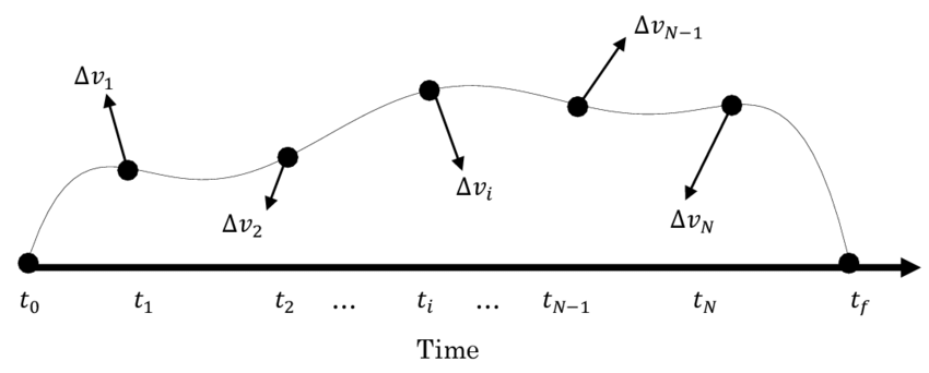
To compute the new velocity vector after the impulsive maneuver, we can add the velocity change vector to the spacecraft’s velocity vector prior to the maneuver:
Similarly, we can compute the position vector after the maneuver using the velocity vector:
where $r_{\text{prior}}$ and ${v}_{\text{prior}}$ represent the spacecraft’s position and velocity vectors before the maneuver, $\Delta t$ is the time interval between maneuvers, and $\Delta {v} \Delta t^2$ represents the contribution of the maneuver to the change in position over the interval.
The impulsive model allows for the formulation of optimization problems where the objective is to find the optimal sequence and magnitude of impulsive maneuvers to achieve specific mission goals, such as reaching a target orbit or minimizing fuel consumption. Constraints can be imposed on the spacecraft’s position, velocity, or acceleration at various points in the trajectory to ensure mission requirements are met.
It is important to note that the impulsive model assumes instantaneous velocity changes and neglects the time required to execute the maneuvers. While this simplification facilitates the optimization process, it may not accurately represent the dynamics of certain spacecraft systems or maneuvers that require finite thrust durations. In such cases, a continuous model, which considers the continuous application of thrust, may be more appropriate.
2.1.2 Continuous Model
The continuous model considers the continuous application of thrust throughout the spacecraft’s trajectory. Unlike the impulsive model, it takes into account the time required to execute the thrust maneuvers and considers variations in thrust magnitude and direction which provides a more detailed representation of the spacecraft’s motion but adds complexity to the optimization problem due to the continuous nature of thrust application.
To describe the continuous model, we can extend the Newtonian equation for the N-body problem. The general representation of continuous transfer is given by the equation:
\begin{equation} \ddot{\mathbf{r}} = -G \sum_{i=1}^{n} \frac{m_i (\mathbf{r} - \mathbf{r}_i)}{|\mathbf{r} - \mathbf{r}_i|^3} + \Gamma \end{equation}
where $\mathbf{r}$ represents the position vector of the spacecraft, $\mathbf{r}_i$ are the positions of $n$ celestial bodies with masses $m_i$, $G$ is the gravitational constant, and $\Gamma$ represents the summation of any accelerations due to sources other than the gravitational force of celestial bodies, such as space perturbations or thrust provided by the spacecraft propulsion system.
By considering the position vector $\mathbf{r}$ and its time derivative $\dot{\mathbf{r}}$ as the state vectors (i.e., $\mathbf{x}(t) = [\mathbf{r} \ \dot{\mathbf{r}}]$), Equation (6) becomes a specific form of the general model representation when considering $\Gamma$ as a function of $\mathbf{u}(t)$. This general equation represents any continuous spacecraft trajectory optimization problem.
By setting $\mathbf{u}(t) = 0$ and considering maneuvers as sudden velocity increments, the continuous model reduces to the impulsive model. However, for specific missions and applications, such as unperturbed orbits around Earth, the orbit propagation may be simplified to orbital elements. Therefore, the complexity of the model can vary for different applications, ranging from simplistic, such as the Hohmann transfer, to highly complicated, such as low-thrust interplanetary transfers.
2.2 Models Based on Equations of Motion
In spacecraft trajectory optimization, various models are employed based on the specific equations of motion that govern the dynamics of the spacecraft. These models provide different levels of accuracy and complexity, depending on the requirements of the mission.
One commonly used model is the two-body problem, which assumes that the spacecraft is influenced only by the gravitational force of a single central body, neglecting the gravitational effects of other celestial bodies. In this model, the spacecraft and central body are considered point masses, and their motion is governed by the following equations of motion:
\begin{equation} \ddot{\mathbf{r}} = -\frac{{\mu}}{{r^3}}\mathbf{r} \end{equation}
where $\ddot{\mathbf{r}}$ is the acceleration vector of the spacecraft, $\mu$ is the gravitational parameter of the central body, $\mathbf{r}$ is the position vector of the spacecraft relative to the central body, and $r$ is the magnitude of $\mathbf{r}$.
To solve the two-body problem, initial conditions, such as the spacecraft’s position and velocity at a specific point in time, are required. From these initial conditions, the spacecraft’s trajectory can be calculated using numerical integration techniques, such as the Runge-Kutta method.
Another model used in spacecraft trajectory optimization is the restricted three-body problem. This model considers the gravitational forces of two primary bodies, typically a planet and its moon or a planet and the Sun, while neglecting the gravitational effects of other celestial bodies. The equations of motion for the restricted three-body problem are more complex and involve additional terms to account for the gravitational influences of both primary bodies.
In addition to these simplified models, more advanced models may be used for specific mission scenarios. These models may consider factors such as atmospheric drag, solar radiation pressure, and perturbations from other celestial bodies. The equations of motion in these cases become more intricate and often require sophisticated numerical techniques for solving.
It is important to note that the choice of the model depends on the specific mission requirements and the level of accuracy desired. Simpler models may be suitable for preliminary analysis or missions with low precision requirements, while more complex models are necessary for high-precision maneuvers and interplanetary missions.
2.2.1 Typical Two-Body Problems
The two-body problem is a fundamental model in spacecraft trajectory optimization, assuming that the spacecraft is influenced solely by the gravitational force of a single celestial body while neglecting gravitational interactions with other bodies. This simplified model allows for the basic formulation of the two-body problem, where the spacecraft’s motion can be described by the equations of motion for a point mass subject to a central gravitational force.
The equations of motion for a spacecraft in a two-body problem can be expressed as follows:
\begin{equation} \ddot{\mathbf{r}} = -\frac{{\mu}}{{r^3}}\mathbf{r} \end{equation}
\begin{equation} \mathbf{r} = \begin{bmatrix} x \ y \ z \end{bmatrix} \end{equation}
where $\ddot{\mathbf{r}}$ represents the acceleration vector of the spacecraft, $\mu$ is the gravitational parameter of the central body, and $\mathbf{r}$ denotes the position vector of the spacecraft relative to the central body. The magnitude of $\mathbf{r}$ is denoted by $r$.
To solve these equations, initial conditions must be provided, specifying the spacecraft’s position and velocity at a particular point in time. These initial conditions are typically obtained from orbital elements or Cartesian coordinates. Numerical integration methods, such as the Runge-Kutta method, can then be employed to propagate the spacecraft’s trajectory.
The two-body problem provides a simplified representation of the spacecraft’s motion around a central body and is particularly useful for analyzing scenarios such as Earth orbits, lunar orbits, or planetary orbits around a single body. However, it does not account for perturbations caused by other celestial bodies, atmospheric drag, or other factors that may affect the spacecraft’s trajectory.
While the two-body problem serves as a valuable starting point for trajectory optimization, more complex models incorporating additional forces and perturbations may be required for precise mission planning and analysis.
Inertial Coordinates
In the case of inertial coordinates, the equations of motion for a two-body problem can be written as:
\begin{equation} m \frac{{d^2 \mathbf{r}}}{{dt^2}} = -\frac{{G M}}{{r^3}} \mathbf{r} \end{equation}
where $G$ is the gravitational constant, $M$ is the mass of the central body, $m$ is the mass of the spacecraft, $\mathbf{r}$ represents the position vector of the spacecraft relative to the central body, and $r$ is the distance between the spacecraft and the central body.
The equation above describes the gravitational force acting on the spacecraft, which is proportional to the product of the masses of the spacecraft and the central body, and inversely proportional to the cube of the distance between them. The negative sign indicates that the force is attractive and directed towards the central body.
Equations of Motion in Scalar and Cylindrical Form
The equations of motion for a spacecraft in a two-body problem can be expressed in scalar form by rewriting the equations derived from the inertial coordinates. This scalar representation provides a set of first-order derivatives:
where $\mu$ is the gravitational constant, $r_x$, $r_y$, and $r_z$ represent the position components ($r = r_x\mathbf{i} + r_y\mathbf{j} + r_z\mathbf{k}$), $v_x$, $v_y$, and $v_z$ are the velocity components ($\mathbf{v} = v_x\mathbf{i} + v_y\mathbf{j} + v_z\mathbf{k}$), and $\gamma_x$, $\gamma_y$, and $\gamma_z$ are the acceleration components ($\mathbf{\gamma} = \gamma_x\mathbf{i} + \gamma_y\mathbf{j} + \gamma_z\mathbf{k}$) in the ECI frame.
In addition to the Cartesian form, cylindrical coordinates are also sometimes considered in research. The equations of motion in cylindrical coordinates can be written as:
where $s = \sqrt{r^2 + z^2}$, and $\gamma_r$, $\gamma_{\theta}$, and $\gamma_z$ represent the acceleration components in cylindrical coordinate systems.
These general equations of motion are widely used in spacecraft trajectory optimization problems [45], particularly for analyzing perturbed orbits [46] and low-thrust transfers [47]. While the Cartesian and cylindrical forms are often employed for typical spacecraft trajectory optimization problems [48], other forms based on the variation of parameters are sometimes utilized in spacecraft trajectory optimization.
To solve this equation, appropriate initial conditions must be provided, specifying the position and velocity of the spacecraft at a particular time. Numerical methods such as numerical integration can then be used to propagate the trajectory of the spacecraft over time.
Inertial coordinates are commonly used in space missions where the central body, such as Earth, is considered fixed in space. These coordinates provide a convenient reference frame for analyzing the motion of the spacecraft relative to distant celestial bodies or for planning interplanetary missions.
It is important to note that the inertial coordinate system assumes a non-rotating and non-accelerating reference frame. While this assumption is valid for short-duration missions and small spatial scales, it may introduce errors for long-duration missions or when considering significant gravitational influences from other celestial bodies.
By considering the inertial coordinates and solving the equations of motion, it is possible to analyze and predict the trajectory of a spacecraft in a two-body problem, providing valuable insights for mission planning and design.
Classical Orbital Elements
Using classical orbital elements, the equations of motion for a two-body problem can be expressed in terms of the orbital elements and their derivatives. These elements provide a more compact representation of the spacecraft’s dynamics and allow for the analysis of orbital perturbations and variations.
The classical orbital elements describe the shape, size, and orientation of an orbit around a central body. They include:
Semi-major axis ($a$): Half of the major axis of the elliptical orbit, representing the average distance between the spacecraft and the central body.
Eccentricity ($e$): A measure of the ellipticity of the orbit, ranging from 0 (circular orbit) to 1 (parabolic orbit).
Inclination ($i$): The angle between the orbital plane and a reference plane, such as the equatorial plane of the central body.
Right ascension of the ascending node ($\Omega$): The angle between the reference direction and the line connecting the central body to the ascending node, where the spacecraft crosses the reference plane from below.
Argument of periapsis ($\omega$): The angle between the ascending node and the periapsis, which is the point in the orbit closest to the central body.
True anomaly ($\nu$): The angle between the periapsis and the spacecraft’s current position in the orbit.
The equations of motion for a two-body problem using classical orbital elements can be expressed as follows:
\begin{equation} \frac{{da}}{{dt}} = \frac{{2}{\sqrt{{\mu}}}{a^2}}{{h}} e \sin{\nu} \frac{{1 + e \cos{\nu}}}{1 - e^2} \end{equation}
\begin{equation} \frac{{de}}{{dt}} = \frac{{\sqrt{{\mu}}}{a^2}}{{h}} \left(\cos{\nu} + e\right) \frac{{\sin{\nu}}}{1 - e^2} \end{equation}
\begin{equation} \frac{{di}}{{dt}} = \frac{{\sqrt{{\mu}}}{a^2}}{{h}} \cos{i} \sin{\nu} \frac{{\sqrt{{1 - e^2}}}}{{1 - e \cos{\nu}}} \end{equation}
\begin{equation} \frac{{d\Omega}}{{dt}} = \frac{{\sqrt{{\mu}}}{a^2}}{{h}} \frac{{\cos{i} \sin{\nu}}}{{\sin{i}}} \frac{{\sqrt{{1 - e^2}}}}{{1 - e \cos{\nu}}} \end{equation}
\begin{equation} \frac{{d\omega}}{{dt}} = \frac{{\sqrt{{\mu}}}{a^2}}{{h}} \frac{{\cos{\nu}}}{{\sin{i}}} \frac{{\sqrt{{1 - e^2}}}}{{1 - e \cos{\nu}}} - \frac{{\sqrt{{\mu}}}{a^2}}{{h e}} \cos{i} \end{equation}
\begin{equation} \frac{{d\nu}}{{dt}} = \frac{{h}}{{r^2}} - \frac{{\sqrt{{\mu}}}{a^2}}{{h}} \frac{{1 + e \cos{\nu}}}{{1 - e^2}} \end{equation}
where $a$, $e$, $i$, $\Omega$, $\omega$, and $\nu$ are the orbital
elements, $\mu$ is the gravitational parameter of the central body, $h$ is the specific angular momentum, and $r$ is the distance between the spacecraft and the central body.
These equations describe the time rate of change of the orbital elements with respect to time. They capture the effects of gravitational forces on the orbit and allow for the analysis of how the orbit evolves over time. By solving these equations, it is possible to predict the variations in the classical orbital elements and understand the long-term behavior of the spacecraft’s trajectory.
The classical orbital elements provide a powerful framework for analyzing and designing spacecraft trajectories, enabling mission planners to determine optimal orbits, evaluate orbital perturbations, and plan maneuvers to achieve desired mission objectives.
Modified Equinoctial Orbital Elements
Similar to the classical orbital elements, the modified equinoctial orbital elements can be used to describe the dynamics of a two-body problem. The modified equinoctial orbital elements offer advantages in terms of numerical stability, making them suitable for optimization and numerical integration purposes. These elements provide a concise representation of the spacecraft’s motion and allow for efficient computations in trajectory optimization.
The modified equinoctial orbital elements include:
Semimajor axis ($a$): Similar to the classical orbital elements, the semimajor axis represents half of the major axis of the elliptical orbit and provides information about the average distance between the spacecraft and the central body.
Eccentricity ($e$): The eccentricity quantifies the ellipticity of the orbit and ranges from 0 (for a circular orbit) to 1 (for a parabolic orbit).
Inclination ($i$): The inclination is the angle between the orbital plane and a reference plane, typically the equatorial plane of the central body.
Longitude of the ascending node ($\Omega$): The longitude of the ascending node specifies the angle between a reference direction and the line connecting the central body to the ascending node, which is the point where the spacecraft crosses the reference plane from below.
Argument of periapsis ($\omega$): The argument of periapsis denotes the angle between the ascending node and the periapsis, which is the point in the orbit closest to the central body.
True longitude ($M$): The true longitude represents the angle between the periapsis and the spacecraft’s current position in the orbit.
The equations of motion for a two-body problem using modified equinoctial orbital elements can be expressed as follows:
\begin{equation} \frac{da}{dt} = \frac{2 \sqrt{\mu}}{n a} f’ \sin f \end{equation}
\begin{equation} \frac{de}{dt} = \frac{\sqrt{\mu}}{n a} \left[(1 - e^2) g + 2 \sqrt{1 - e^2} h \cos f\right] \end{equation}
\begin{equation} \frac{di}{dt} = \frac{\sqrt{\mu}}{n a} \left[\frac{\sqrt{1 - e^2}}{1 + e \cos f} k \sin f\right] \end{equation}
\begin{equation} \frac{d\Omega}{dt} = \frac{\sqrt{\mu}}{n a} \left[\frac{\sqrt{1 - e^2}}{1 + e \cos f} k \frac{\sin f}{\sin i}\right] \end{equation}
\begin{equation} \frac{d\omega}{dt} = \frac{\sqrt{\mu}}{n a} \left[\frac{\sqrt{1 - e^2}}{1 + e \cos f} (k \cos \omega - h \sin \omega) - \frac{e}{1 - e^2} \cos i\right] \end{equation}
\begin{equation} \frac{dM}{dt} = n + \frac{\sqrt{\mu}}{n a} \left[(1 - e^2) g + 2 \sqrt{1 - e^2} h \cos f\right] \end{equation}
where $n$ is the mean motion and represents the rate of change of the mean anomaly, $f$ is the true anomaly,
and $\mu$ is the gravitational parameter of the central body.
These equations describe the time rate of change of the modified equinoctial orbital elements. By numerically integrating these equations, it is possible to propagate the spacecraft’s orbit and analyze its dynamics over time. The modified equinoctial orbital elements provide a robust and efficient framework for trajectory optimization and numerical simulations in space mission design.
2.2.2 Rendezvous
Rendezvous trajectories involve the precise alignment of two spacecraft in space. The mathematical models for rendezvous trajectories consider the relative motion between the chaser and target spacecraft and aim to find optimal trajectories that minimize the distance and time required for the rendezvous. These models incorporate additional constraints, such as avoiding collisions and satisfying docking requirements.
2.2.3 Libration points
Libration points, also known as Lagrange points, are positions in space where the gravitational forces of two celestial bodies balance the centripetal force felt by a smaller object. The mathematical models for libration point trajectories analyze the motion of spacecraft in the vicinity of these points, taking into account the gravitational forces and the stability characteristics of the libration points.
By employing these mathematical models, spacecraft trajectory optimization can be approached from different perspectives and tailored to the specific requirements of the mission. These models provide a foundation for formulating the optimization problem and developing algorithms to find optimal trajectories that satisfy mission objectives and constraints.
3. Optimization Algorithms
Spacecraft trajectory optimization can be approached using different algorithms. Here, we will focus on two main categories: direct methods and indirect methods.
3.1 Direct Methods
Direct methods transform the optimization problem into a parameter optimization problem and solve it directly. Two commonly used direct methods are single-shooting and multiple-shooting.
3.1.1 Single-Shooting
In single-shooting, the entire trajectory is parameterized, and the problem is transformed into a parameter optimization problem. The trajectory is divided into smaller segments, and the state and control variables are approximated within each segment. The optimization algorithm optimizes the parameters to find the best trajectory.
To implement single-shooting in Python, you can use techniques such as gradient-based optimization algorithms (e.g., gradient descent, Newton’s method) or derivative-free optimization algorithms (e.g., genetic algorithms, particle swarm optimization).
3.1.2 Multiple-Shooting
Multiple-shooting is an extension of single-shooting, where the trajectory is divided into smaller segments, but the state and control variables are defined at the segment boundaries. This method allows for more accurate approximations of the dynamics and can lead to better convergence.
To implement multiple-shooting in Python, you can use shooting methods combined with numerical integration techniques (e.g., Runge-Kutta methods) to propagate the state from one segment boundary to the next. The optimization algorithm then adjusts the control variables to find the optimal trajectory.
3.2 Indirect Methods
Indirect methods transform the trajectory optimization problem into a two-point boundary value problem (TPBVP). The TPBVP is then solved using optimization techniques such as Pontryagin’s minimum principle or variational methods.
3.2.1 Pontryagin’s Minimum Principle
Pontryagin’s minimum principle is a powerful tool for solving optimal control problems. It provides necessary conditions for optimality in terms of a set of differential equations called the Hamiltonian equations. Solving these equations can yield the optimal control and state trajectories.
To implement Pontryagin’s minimum principle in Python, you can use techniques such as numerical shooting methods or indirect optimization algorithms (e.g., sequential quadratic programming) to solve the associated boundary value problem.
3.2.2 Variational Methods
Variational methods approach trajectory optimization as a calculus of variations problem. The problem is transformed into finding the trajectory that minimizes a cost functional, subject to the dynamics and boundary conditions. Euler-Lagrange equations are derived and solved to find the optimal trajectory.
To implement variational methods in Python, you can use techniques such as the Euler-Lagrange equation solver or direct collocation methods. These methods typically involve discretizing the trajectory and formulating the optimization problem as a nonlinear programming problem.
4. Implementation in Python
4.1 Setting up the Environment
To begin the implementation, set up your Python environment with the necessary libraries. Make sure you have NumPy, SciPy, and matplotlib installed. Additionally, you may need to install specific libraries for optimization algorithms, such as scipy.optimize or third-party libraries like pyOpt or GPOPS-II depending on your chosen approach.
import numpy as np
from scipy.integrate import solve_bvp
import matplotlib.pyplot as plt
4.2 Problem Formulation
Next, define the mission parameters, decision variables, objective function, and constraints based on your specific scenario.
# Define mission parameters
departure_location = [0, 0, 0]  # XYZ coordinates
arrival_location = [100, 200, 300]  # XYZ coordinates
departure_time = 0
arrival_time = 100

# Define decision variables
thrust_direction = [1, 0, 0]  # Unit vector
thrust_magnitude = 1.0  # N

# Define objective function


def objective_function(x, u, t):
    # Define your objective function here
    pass

# Define constraints
def constraints(x, u, t):
    # Define your constraints here
    pass
4.3 Optimization Algorithm Implementation
Choose the optimization algorithm that suits your problem and implement it using the defined mission parameters, decision variables, objective function, and constraints. Here are some general steps for implementation:
- Define the optimization problem using appropriate syntax or mathematical modeling tools.
- Specify the objective function and constraints based on the problem formulation.
- Select an appropriate optimization algorithm and configure its parameters.
- Run the optimization algorithm on the defined problem and obtain the optimized solution.
- Extract and interpret the optimized trajectory, control inputs, and other relevant information.
# Implement your optimization algorithm here
4.4 Visualizing and Analyzing the Results
Once the optimization algorithm has converged, visualize and analyze the optimized trajectories using Python’s plotting libraries.
# Visualize the optimized trajectories
plt.figure(figsize=(10, 6))
plt.plot(x_opt, y_opt, 'r-', label='Optimal Trajectory')
plt.xlabel('X')
plt.ylabel('Y')
plt.title('Optimized Spacecraft Trajectory')
plt.legend()
plt.grid(True)
plt.show()
You can customize the visualization to include other relevant information, such as control inputs, time evolution, or specific mission constraints.
Conclusion
In this comprehensive tutorial, we explored advanced techniques for spacecraft trajectory optimization using Python. We covered problem formulation, various optimization algorithms, and their implementation in Python. By combining theoretical knowledge of astrodynamics and optimization with practical programming skills, you can effectively tackle complex trajectory optimization problems in the aerospace industry. Experiment with different algorithms, problem setups, and optimization parameters to enhance your understanding and skills in this field. Remember to consider the specific characteristics and requirements of your mission to achieve meaningful and realistic results.
Arman Asgharpoor Golroudbari
Machine Learning Engineer
Machine Learning Engineer with 5+ years of experience in LLMs, transformer architectures, computer vision systems, and autonomous robotics.