OxIOD IMU Dataset

Oct 29, 2022 8 min read

OxIOD Dataset
How to use OxIOD Dataset
Use OxIOD Dataset in Python
References

OxIOD Dataset

Oxford Inertial Odometry Dataset [1] is a large set of inertial data for inertial odometry which is recorded by smartphones at 100 Hz in indoor environment. The suite consists of 158 tests and covers a distance of over 42 km, with OMC ground track available for 132 tests. Therefore, it does not include pure rotational movements and pure translational movements, which are helpful for systematically evaluating the model’s performance under different conditions; however, it covers a wide range of everyday movements.

Due to the different focus, some information (for example, the alignment of the coordinate frames) is not accurately described. In addition, the orientation of the ground trace contains frequent irregularities (e.g., jumps in orientation that are not accompanied by similar jumps in the IMU data). The dataset is available at Link.

How to use OxIOD Dataset

The dataset can be download from here. The Dataset Contains:

24 Handheld Sequences

Total 8821 seconds for 7193 meters.

data1	time (s)	distance (m)
seq1	376	301
seq2	234	177
seq3	188	147
seq4	216	166
seq5	322	264
seq6	325	274
seq7	141	118
total	1802	1447

data2	time (s)	dis (m)
seq1	326	281
seq2	312	264
seq3	301	249
total	939	794

data3	time	dis
seq1	308	251
seq2	379	324
seq3	609	533
seq4	538	467
seq5	383	319
total	2217	1894

data4	time	dis
seq1	317	242
seq2	322	243
seq3	606	476
seq4	438	359
seq5	350	284
total	2033	1604

data5	time	dis
seq1	310	237
seq2	594	466
seq3	560	445
seq4	366	306
total	1830	1454

11 Pocket Sequences

Total 5622 seconds for 4231 meters.

data1	time	dis
seq1	330	284
seq2	456	379
seq3	506	405
seq4	491	387
seq5	240	182
total	2023	1637

data2	time	dis
seq1	651	492
seq2	559	414
seq3	628	429
seq4	668	494
seq5	470	371
seq6	623	494
total	3599	2694

8 Handbag Sequences

Total 4100 seconds for 3431 meters.

data1	time	dis
seq1	575	437
seq2	570	467
seq3	580	466
seq4	445	366
total	2170	1736

data2	time	dis
seq1	575	487
seq2	560	499
seq3	425	381
seq4	370	328
total	1930	1695

13 Trolley Sequences

Total 4262 seconds for 2685 meters.

data1	time	dis
seq1	447	251
seq2	309	169
seq3	359	209
seq4	599	362
seq5	612	374
seq6	586	380
seq7	274	174
total	3186	1919

data2	time	dis
seq1	156	106
seq2	168	118
seq3	161	113
seq4	163	113
seq5	217	158
seq6	211	158
total	1076	766

8 Slow Walking Sequences

Total 4150 seconds for 2421 meters.

data1	time	dis
seq1	612	382
seq2	603	353
seq3	617	341
seq4	594	323
seq5	606	352
seq6	503	331
seq7	311	172
seq8	304	167
total	4150	2421

7 Running Sequences

Total 3732 seconds for 4356 meters.

data1	time	dis
seq1	691	761
seq2	623	719
seq3	590	665
seq4	603	679
seq5	619	766
seq6	303	373
seq7	303	393
total	3732	4356

26 Multi Devices Sequences

Total 7144 seconds for 5350 meters.

iPhone 5	time	dis
seq1	178	150
seq2	163	133
seq3	160	126
seq4	124	100
seq5	174	139
seq6	167	136
seq7	197	150
seq8	184	141
seq9	184	142
total	1531	1217

iPhone 6	time	dis
seq1	180	165
seq2	184	171
seq3	182	168
seq4	150	140
seq5	183	162
seq6	171	155
seq7	184	139
seq8	185	148
seq9	173	133
total	1592	1381

nexus 5	time	dis
seq1	604	452
seq2	609	438
seq3	605	414
seq4	609	403
seq5	607	388
seq6	607	401
seq7	186	130
seq8	194	127
total	4021	2752

35 Multi Users Sequences

Total 8821 seconds for 9465 meters.

user 2	time	dis
seq1	311	284
seq2	358	313
seq3	390	328
seq4	217	172
seq5	311	240
seq6	256	193
seq7	371	296
seq8	450	375
seq9	264	221
total	2928	2422

user 3	time	dis
seq1	382	301
seq2	318	272
seq3	340	295
seq4	232	198
seq5	214	185
seq6	356	289
seq7	258	203
total	2100	1743

user 4	time	dis
seq1	387	367
seq2	329	307
seq3	305	288
seq4	248	229
seq5	356	314
seq6	293	272
seq7	297	260
seq8	468	411
seq9	435	364
total	3118	2812

user 5	time	dis
seq1	294	237
seq2	305	264
seq3	253	211
seq4	390	337
seq5	300	226
seq6	338	284
seq7	168	154
seq8	410	395
seq9	274	250
seq10	152	130
total	2884	2488

26 Large Scale Sequences

Total 4161 seconds for 3465 meters.

floor1	time	dis
seq1	153	142
seq2	165	143
seq3	158	142
seq4	157	145
seq5	156	142
seq6	156	142
seq7	161	144
seq8	155	143
seq9	160	126
seq10	158	143
total	1579	1412

floor4	time	dis
seq1	160	170
seq2	157	153
seq3	162	153
seq4	118	106
seq5	164	153
seq6	163	143
seq7	169	141
seq8	166	153
seq9	172	135
seq10	169	154
seq11	166	152
seq12	165	154
seq13	165	133
seq14	164	153
seq15	163	153
seq16	159	133
total	2582	2053

In each folder, there is a raw data subfolder and a syn data subfolder, which represent the raw data collection without synchronisation but with high precise timestep, and the synchronised data but without high precise timestep.

The header of files is

vicon (vi.csv)*

Time
Header
translation.x translation.y translation.z
rotation.x rotation.y rotation.z rotation.w

Sensors (imu.csv)*

Time
attitude_roll(radians) attitude_pitch(radians) attitude_yaw(radians)
rotation_rate_x(radians/s) rotation_rate_y(radians/s) rotation_rate_z(radians/s)
gravity_x(G) gravity_y(G) gravity_z(G)
user_acc_x(G) user_acc_y(G) user_acc_z(G)
magnetic_field_x(microteslas) magnetic_field_y(microteslas) magnetic_field_z(microteslas)

Use OxIOD Dataset in Python

First, we need to import libraries

import numpy as np
import pandas as pd
import matplotlib.pyplot as plt

Create variables to store data

imu_data_OxIOD =[]
gt_data_OxIOD = []
imu = np.zeros((1,9))
gt = np.zeros((1,7))

Load data files

imu_data_OxIOD.append(
    'handheld/data5/syn/imu3.csv')
imu_data_OxIOD.append(
    'handheld/data2/syn/imu1.csv')
imu_data_OxIOD.append(
    'handheld/data2/syn/imu2.csv')
imu_data_OxIOD.append(
    'handheld/data5/syn/imu2.csv')
imu_data_OxIOD.append(
    'handheld/data3/syn/imu4.csv')
imu_data_OxIOD.append(
    'handheld/data4/syn/imu4.csv')
imu_data_OxIOD.append(
    'handheld/data4/syn/imu2.csv')
imu_data_OxIOD.append(
    'handheld/data1/syn/imu7.csv')
imu_data_OxIOD.append(
    'handheld/data5/syn/imu4.csv')
imu_data_OxIOD.append(
    'handheld/data4/syn/imu5.csv')
imu_data_OxIOD.append(
    'handheld/data1/syn/imu3.csv')
imu_data_OxIOD.append(
    'handheld/data3/syn/imu2.csv')
imu_data_OxIOD.append(
    'handheld/data2/syn/imu3.csv')
imu_data_OxIOD.append(
    'handheld/data1/syn/imu1.csv')
imu_data_OxIOD.append(
    'handheld/data3/syn/imu3.csv')
imu_data_OxIOD.append(
    'handheld/data3/syn/imu5.csv')
imu_data_OxIOD.append(
    'handheld/data1/syn/imu4.csv')

gt_data_OxIOD.append(
    'handheld/data5/syn/vi3.csv')
gt_data_OxIOD.append(
    'handheld/data2/syn/vi1.csv')
gt_data_OxIOD.append(
    'handheld/data2/syn/vi2.csv')
gt_data_OxIOD.append(
    'handheld/data5/syn/vi2.csv')
gt_data_OxIOD.append(
    'handheld/data3/syn/vi4.csv')
gt_data_OxIOD.append(
    'handheld/data4/syn/vi4.csv')
gt_data_OxIOD.append(
    'handheld/data4/syn/vi2.csv')
gt_data_OxIOD.append(
    'handheld/data1/syn/vi7.csv')
gt_data_OxIOD.append(
    'handheld/data5/syn/vi4.csv')
gt_data_OxIOD.append(
    'handheld/data4/syn/vi5.csv')
gt_data_OxIOD.append(
    'handheld/data1/syn/vi3.csv')
gt_data_OxIOD.append(
    'handheld/data3/syn/vi2.csv')
gt_data_OxIOD.append(
    'handheld/data2/syn/vi3.csv')
gt_data_OxIOD.append(
    'handheld/data1/syn/vi1.csv')
gt_data_OxIOD.append(
    'handheld/data3/syn/vi3.csv')
gt_data_OxIOD.append(
    'handheld/data3/syn/vi5.csv')
gt_data_OxIOD.append(
    'handheld/data1/syn/vi4.csv')

Import data from file

for i, (imu_data_filename, gt_data_filename) in enumerate(zip(imu_data_OxIOD, gt_data_OxIOD)):
        oxiod_gt    = pd.read_csv(gt_data_filename).values
        oxiod_imu   = pd.read_csv(imu_data_filename).values
        oxiod_imu   = np.hstack([oxiod_imu[:, 10:13], oxiod_imu[:, 4:7], oxiod_imu[:, 7:10]])
        oxiod_gt = np.hstack([np.concatenate([oxiod_gt[:, 8:9], oxiod_gt[:, 5:8]], axis=1), oxiod_gt[:, 2:5]])
        imu = np.vstack([imu, oxiod_imu])
        gt = np.vstack([gt,oxiod_gt])
acc = imu[:,0:3]
gyro =imu[:,3:6]
mag = imu[:,6:9]
ori = gt[:,0:4]
pose = gt[:,4:7]

Store in csv file

df_imu = pd.DataFrame({'Acc x': acc[1:, 0], 'Acc y': acc[1:, 1], 'Acc z': acc[1:, 2], 'Gyro x': gyro[1:, 0],
                      'Gyro y': gyro[1:, 1], 'Gyro z': gyro[1:, 2], 'Mag x': mag[1:, 0], 'Mag y': mag[1:, 1], 'Mag z': mag[1:, 2]})
df_imu.to_csv('OxIOD_IMU_train.csv', index=False)
df_gt = pd.DataFrame({'Ori w': ori[1:, 0], 'Ori x': ori[1:, 1], 'Ori y': ori[1:, 2],
                     'Ori z': ori[1:, 3], 'Pose x': pose[1:, 0], 'Pose y': pose[1:, 1], 'Pose z': pose[1:, 2]})
df_gt.to_csv('OxIOD_GT_train.csv', index=False)

The data could be plot by

import matplotlib.pyplot as plt
fs = 100
dt = 1/fs
t = np.arange(0, acc.shape[0]/fs, dt)

# Plot the IMU readings
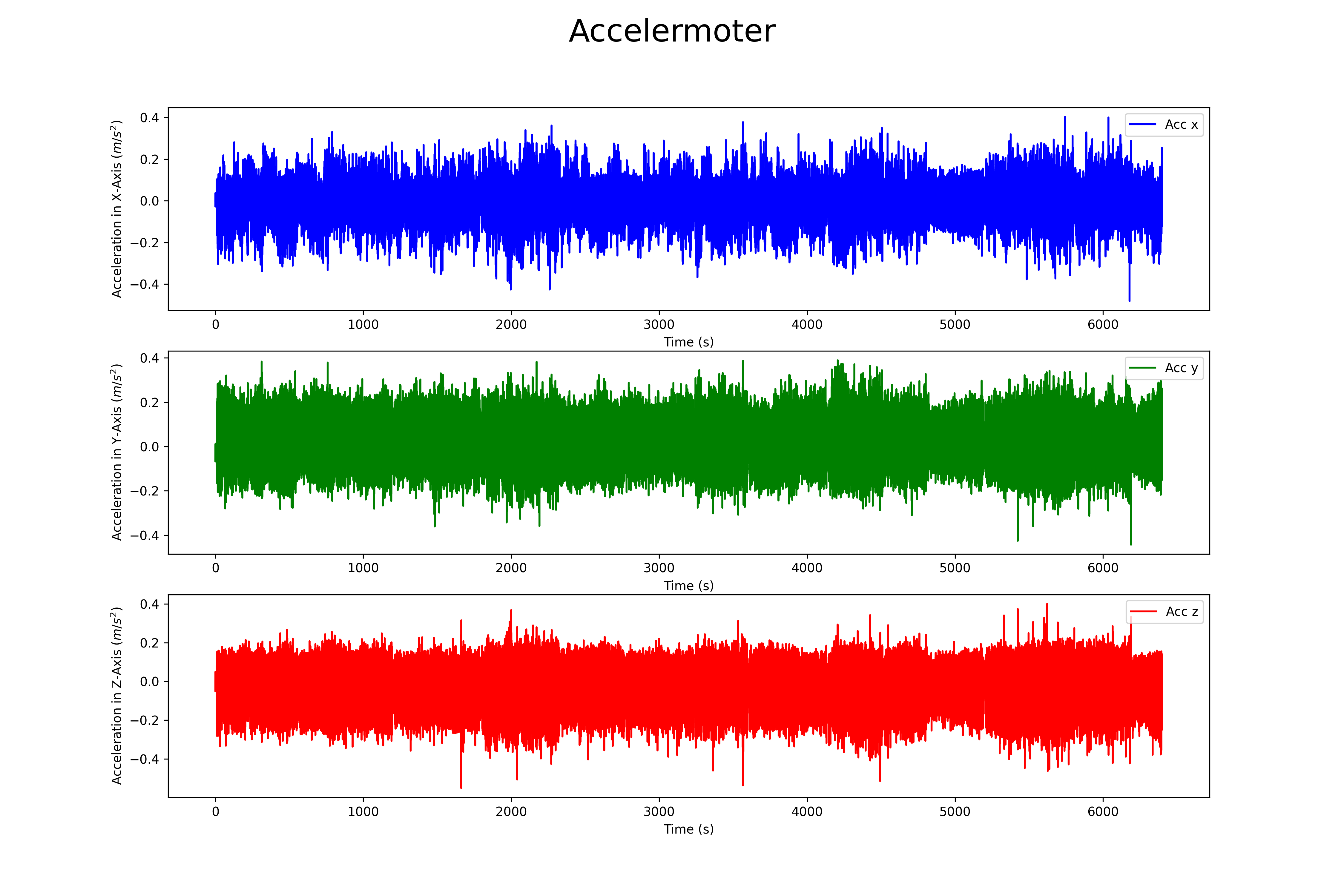
## Accelermoter 
# Plotting the three axis of the accelerometer in one figure.
plt.figure(figsize=(15, 10))
plt.subplot(3, 1, 1)
plt.plot(t, acc[:, 0], label='Acc x', color='b')
plt.legend(loc="upper right")
plt.xlabel('Time (s)')
plt.ylabel('Acceleration in X-Axis ($m/s^2$)')
plt.subplot(3, 1, 2)
plt.plot(t, acc[:, 1], label='Acc y', color='g')
plt.legend(loc="upper right")
plt.xlabel('Time (s)')
plt.ylabel('Acceleration in Y-Axis ($m/s^2$)')
plt.subplot(3, 1, 3)
plt.plot(t, acc[:, 2], label='Acc z', color='r')
plt.xlabel('Time (s)')
plt.ylabel('Acceleration in Z-Axis ($m/s^2$)')
plt.legend(loc="upper right")
plt.suptitle("Accelermoter", fontsize=25)
plt.savefig('RIDI_Acc.png', dpi=300)

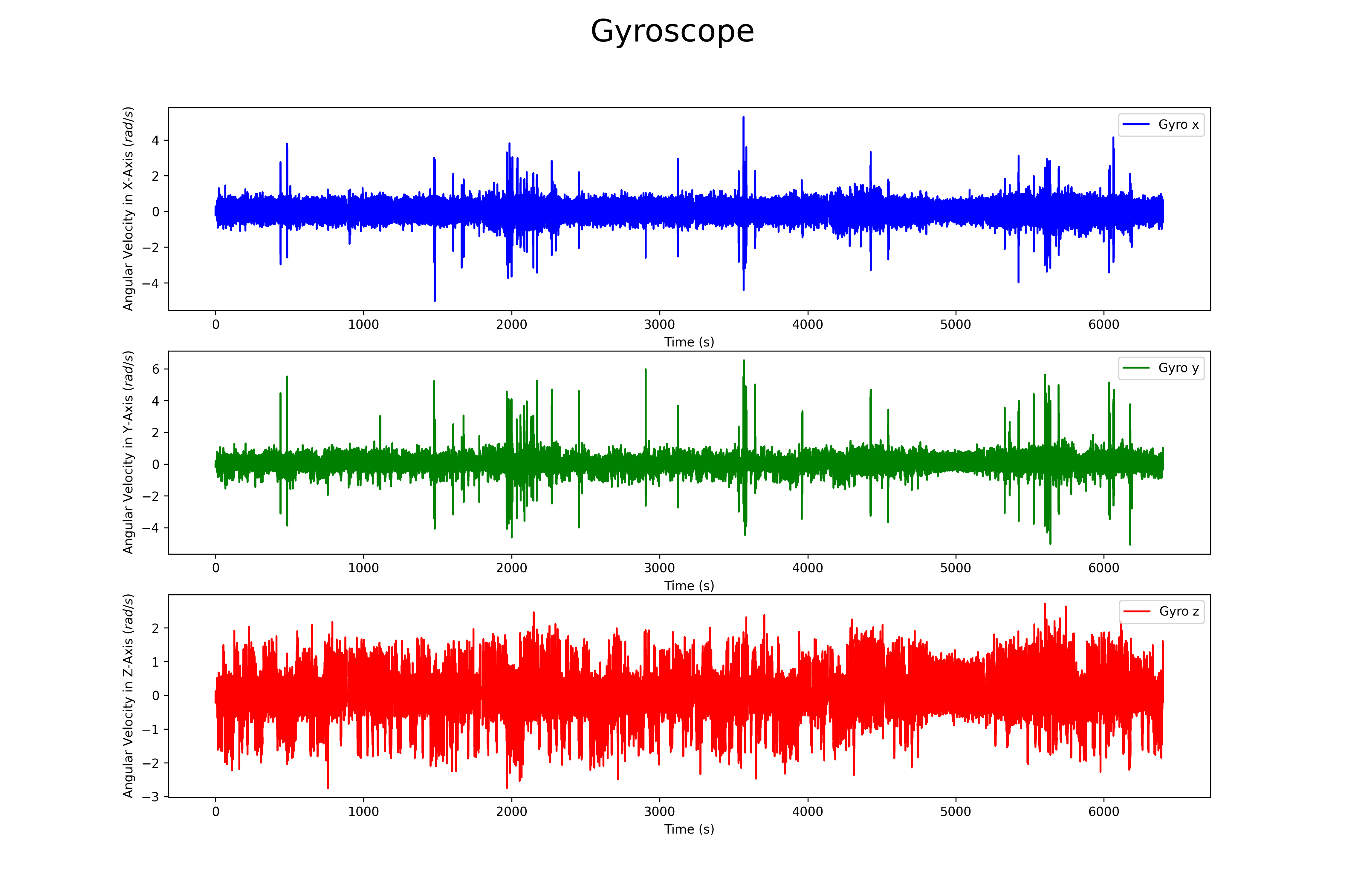
## Gyroscope 
# Plotting the three axis of the gyroscope in one figure.
plt.figure(figsize=(15, 10))
plt.subplot(3, 1, 1)
plt.plot(t, gyro[:, 0], label='Gyro x', color='b')
plt.legend(loc="upper right")
plt.xlabel('Time (s)')
plt.ylabel('Angular Velocity in X-Axis ($rad/s$)')
plt.subplot(3, 1, 2)
plt.plot(t, gyro[:, 1], label='Gyro y', color='g')
plt.legend(loc="upper right")
plt.xlabel('Time (s)')
plt.ylabel('Angular Velocity in Y-Axis ($rad/s$)')
plt.subplot(3, 1, 3)
plt.plot(t, gyro[:, 2], label='Gyro z', color='r')
plt.xlabel('Time (s)')
plt.ylabel('Angular Velocity in Z-Axis ($rad/s$)')
plt.legend(loc="upper right")
plt.suptitle("Gyroscope", fontsize=25)
plt.savefig('RIDI_Gyro.png', dpi=300)

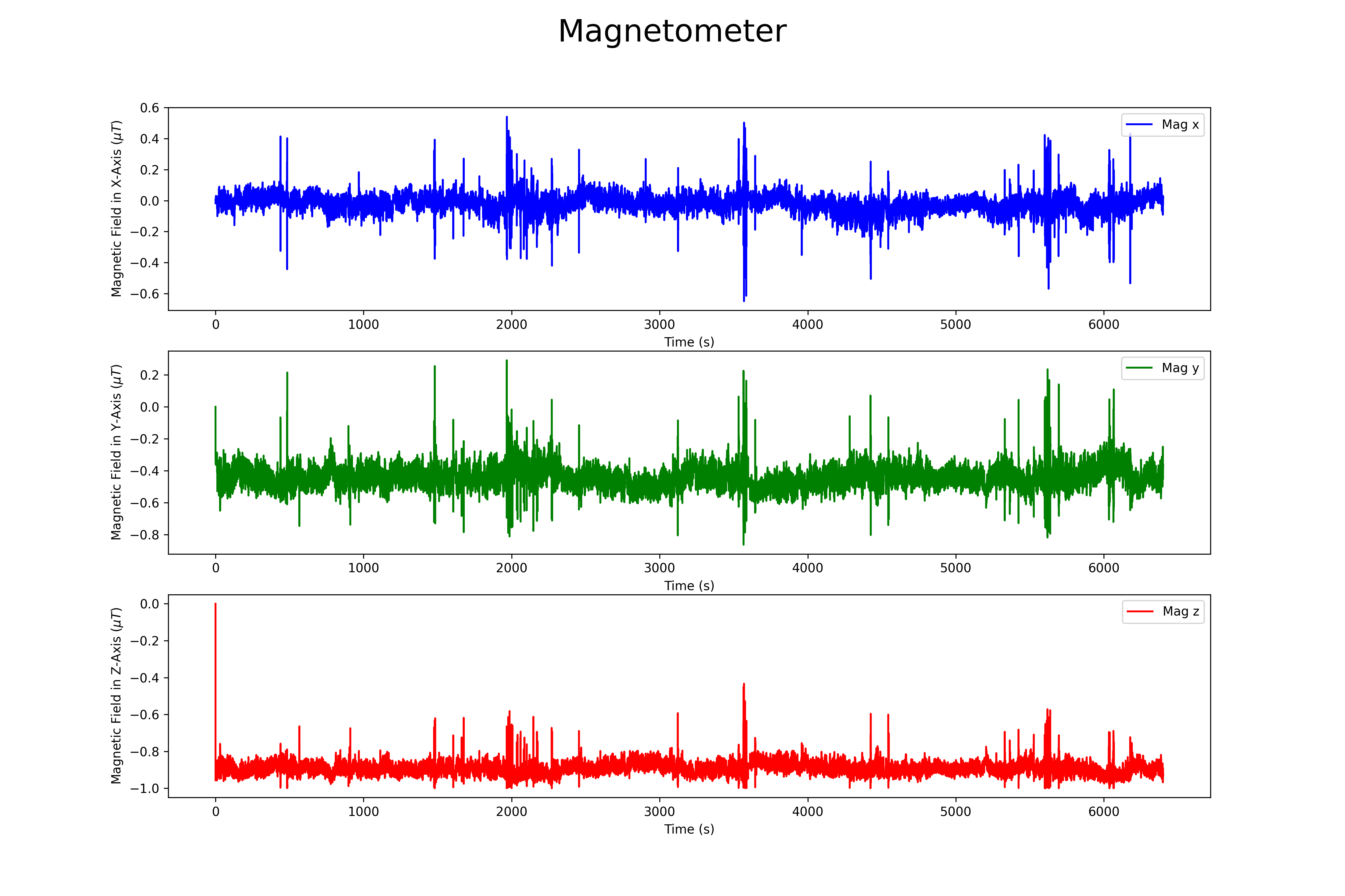
## Magnetometer
# Plotting the three axis of the magnetometer in one figure.
plt.figure(figsize=(15, 10))
plt.subplot(3, 1, 1)
plt.plot(t, mag[:, 0], label='Mag x', color='b')
plt.legend(loc="upper right")
plt.xlabel('Time (s)')
plt.ylabel('Magnetic Field in X-Axis ($\mu T$)')
plt.subplot(3, 1, 2)
plt.plot(t, mag[:, 1], label='Mag y', color='g')
plt.legend(loc="upper right")
plt.xlabel('Time (s)')
plt.ylabel('Magnetic Field in Y-Axis ($\mu T$)')
plt.subplot(3, 1, 3)
plt.plot(t, mag[:, 2], label='Mag z', color='r')
plt.xlabel('Time (s)')
plt.ylabel('Magnetic Field in Z-Axis ($\mu T$)')
plt.legend(loc="upper right")
plt.suptitle("Magnetometer", fontsize=25)
plt.savefig('RIDI_Mag.png', dpi=300)

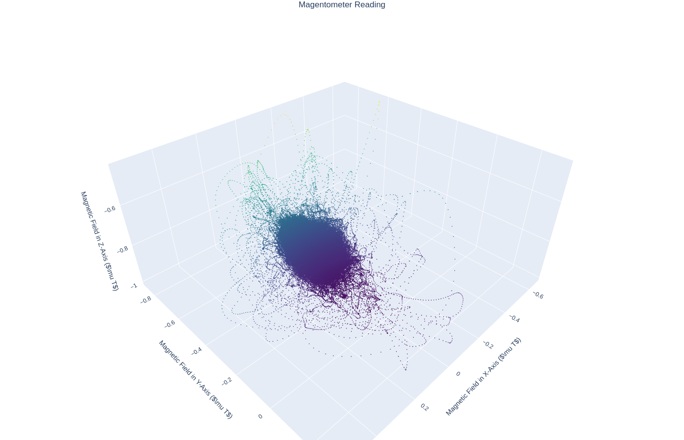
The magnetomer 3d scatter plot can be found here

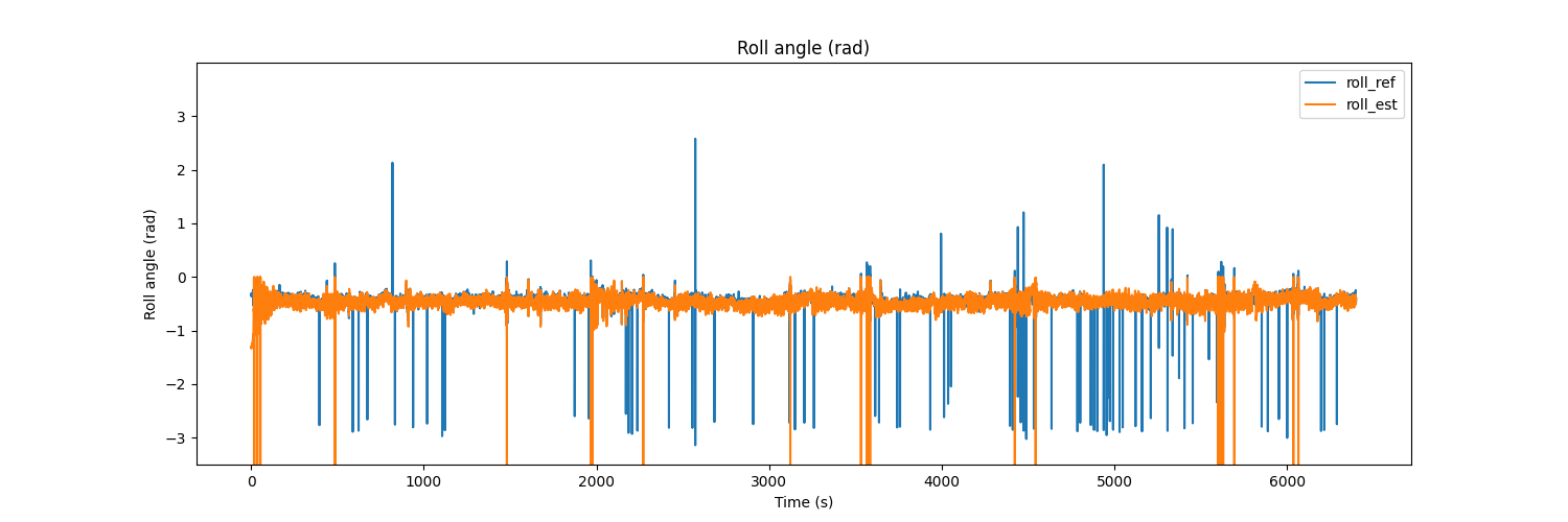
To test the dataset, we can use AHRS [2] library which has multiple sensor fusion algorithm for python. The Madgwick algorithm has been chosen as SFA.

fs = 100
dt = 1/fs
t = np.arange(0, acc.shape[0]/fs, dt)
madgwick = sfa.Madgwick(gyr=gyro, acc=acc, mag=mag, frequency=fs)

roll_ref, pitch_ref, yaw_ref = quat2eul(ori)
roll_est, pitch_est, yaw_est = quat2eul(madgwick.Q)

# Plot the results
# Roll
plt.figure(figsize=(15, 5))
plt.plot(t, roll_ref, label='roll_ref')
plt.plot(t, roll_est, label='roll_est')
plt.title('Roll angle (rad)')
plt.xlabel('Time (s)')
plt.ylabel('Roll angle (rad)')
plt.ylim(-3.5, 3.999)
plt.legend(loc='upper right')
plt.show()
# Pitch
plt.figure(figsize=(15, 5))
plt.plot(t, pitch_ref, label='pitch_ref')
plt.plot(t, pitch_est, label='pitch_est')
plt.title('Pitch angle (rad)')
plt.xlabel('Time (s)')
plt.ylabel('Pitch angle (rad)')
plt.ylim(-3.5, 3.999)
plt.legend(loc='upper right')
plt.show()
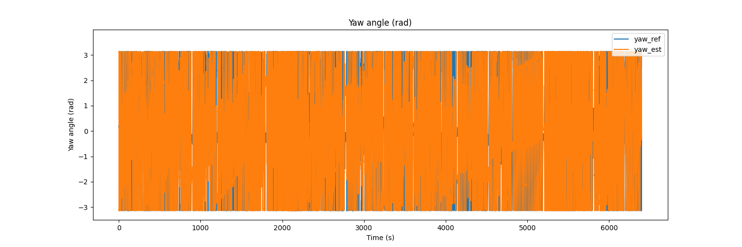
# Yaw
plt.figure(figsize=(15, 5))
plt.plot(t, yaw_ref, label='yaw_ref')
plt.plot(t, yaw_est, label='yaw_est')
plt.title('Yaw angle (rad)')
plt.xlabel('Time (s)')
plt.ylabel('Yaw angle (rad)')
plt.ylim(-3.5, 3.999)
plt.legend(loc='upper right')
plt.show()

The result would be as follows Roll Pitch Yaw

Dataset

References

[1] C. Chen, P. Zhao, C. X. Lu, W. Wang, A. Markham, and N. Trigoni, “Oxiod: The dataset for deep inertial odometry,” arXiv preprint arXiv:1809.07491, 2018. Link

[2] ahrs.readthedocs.io/en