KITTI Dataset
- Introduction
- Data Format
- Downloading the Dataset
- Using the KITTI Dataset in Python
- Understanding Calibration and Timestamp Data in 3D Vision Applications
- Processing Image Data with Timestamps
- Depth Maps and Visual Odometry
- Calculating Baseline and Focal Length in Stereo Vision
- Calculating Depth from Stereo Pair of Images
- Math behind Stereo Depth
- Feature Extraction
- Feature Matching
- References
Introduction
KITTI is a popular computer vision dataset designed for autonomous driving research. It contains a diverse set of challenges for researchers, including object detection, tracking, and scene understanding. The dataset is derived from the autonomous driving platform developed by the Karlsruhe Institute of Technology and the Toyota Technological Institute at Chicago.
The KITTI dataset includes a collection of different sensors and modalities, such as stereo cameras, LiDAR, and GPS/INS sensors, which provides a comprehensive view of the environment around the vehicle. The data was collected over several days in the urban areas of Karlsruhe and nearby towns in Germany. The dataset includes more than 200,000 stereo images and their corresponding point clouds, as well as data from the GPS/INS sensors, which provide accurate location and pose information.
The dataset is divided into several different categories, each with its own set of challenges. These categories include object detection, tracking, scene understanding, visual odometry, and road/lane detection. Each category contains a set of challenges that researchers can use to evaluate their algorithms and compare their results with others in the field.
One of the strengths of the KITTI dataset is its accuracy and precision. The sensors used to collect the data provide a high level of detail and accuracy, making it possible to detect and track objects with high precision. Additionally, the dataset includes a large number of real-world scenarios, which makes it more representative of real-world driving conditions.
Another strength of the KITTI dataset is its large size. The dataset includes over 50 GB of data, which includes stereo images, point clouds, and GPS/INS data. This large amount of data makes it possible to train deep neural networks, which are known to perform well on large datasets.
Despite its strengths, the KITTI dataset also has some limitations. For example, the dataset only covers urban driving scenarios, which may not be representative of driving conditions in other environments. Additionally, the dataset is relatively small compared to other computer vision datasets, which may limit its applicability in certain domains.
In summary, the KITTI dataset is a valuable resource for researchers in the field of autonomous driving. Its accuracy, precision, and large size make it an ideal dataset for evaluating and comparing algorithms for object detection, tracking, and scene understanding. While it has some limitations, its strengths make it a popular and widely used dataset in the field.
Data Format
The KITTI dataset is available in two formats: raw data and preprocessed data. The raw data contains a large amount of sensor data, including images, LiDAR point clouds, and GPS/IMU measurements, and can be used for various research purposes. The preprocessed data provides more structured data, including object labels, and can be used directly for tasks such as object detection and tracking.
Downloading the Dataset
The KITTI dataset can be downloaded from the official website (http://www.cvlibs.net/datasets/kitti/) after registering with a valid email address. The website provides instructions on how to download and use the data, including the required software tools and file formats.
Using the KITTI Dataset in Python
Prerequisites
Before getting started, make sure you have the following prerequisites:
- Python 3.x installed
- NumPy and Matplotlib libraries installed
- KITTI dataset downloaded and extracted
- OpenCV: for image and video processing
- Pykitti: a Python library for working with the KITTI dataset
Install the Required Libraries
Once you have downloaded the dataset, you will need to install the required libraries to work with it in Python. The following libraries are commonly used:
NumPy: for numerical operations and array manipulation OpenCV: for image and video processing Matplotlib: for data visualization You can install these libraries using pip, the Python package manager, by running the following commands in your terminal:
pip install numpy
pip install opencv-python
pip install matplotli
pip install plotly
pip install glob
pip install progressbar
Load the Dataset
The KITTI Odometry dataset consists of multiple sequences, each containing a set of stereo image pairs and corresponding ground truth poses. We will load the data using the cv2 library in Python.
# Import the libraries
import numpy as np
import cv2
import os
import glob
import pandas as pd
import matplotlib.pyplot as plt
import plotly.graph_objects as go

# Define the paths to the data
path_img = "./data_odometry_gray/dataset/sequences/"
path_pose = "./data_odometry_poses/dataset/poses/"

# Load the pose data using pandas
num = "00"
poses = pd.read_csv(path_pose + ("%s.txt" % num), delimiter=' ', header=None)

# Extract the ground truth coordinates from the pose data
gt = np.array([np.array(poses.iloc[i]).reshape((3, 4)) for i in range(len(poses))])

# Extracting spatial coordinates from the gt tensor
z = gt[:, :, 3][:, 2]
y = gt[:, :, 3][:, 1]
x = gt[:, :, 3][:, 0]

# Creating a 3D scatter plot using Plotly
fig = go.Figure(data=[go.Scatter3d(
    x=x,
    y=y,
    z=z,
    mode='lines',
    line=dict(color='red', width=2)
)])

# Customize the layout of the plot
fig.update_layout(scene=dict(
    xaxis_title='X',
    yaxis_title='Y',
    zaxis_title='Z',
    camera=dict(
        eye=dict(x=1.5, y=1.5, z=0.6),
        projection=dict(type='perspective')
    ),
    bgcolor='whitesmoke',
    xaxis=dict(showgrid=True, gridwidth=0.8, gridcolor='lightgray'),
    yaxis=dict(showgrid=True, gridwidth=0.8, gridcolor='lightgray'),
    zaxis=dict(showgrid=True, gridwidth=0.8, gridcolor='lightgray')
))

# Add a title to the plot for better context
fig.update_layout(title='Spatial Trajectory', title_font=dict(size=16, color='black'))

# Display the spatial trajectory plot
fig.show()
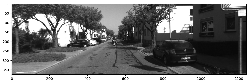
# Load and display a test image
test_img = cv2.imread(path_img + num + '/image_0/000000.png')
plt.figure(figsize=(12, 6))
plt.imshow(test_img)
plt.axis('off')
plt.title('Test Image')
plt.show()
Understanding Calibration and Timestamp Data in 3D Vision Applications
In 3D vision applications, accurate calibration and synchronized timestamps play a crucial role in aligning and mapping data from multiple sensors. In following, we will explore the contents of two important files: calib.txt and times.txt. These files provide essential information for camera calibration and synchronization of image pairs. Understanding these concepts is vital for accurately transforming and processing data in 3D vision applications.
In computer vision and camera calibration, intrinsic and extrinsic matrices are used to describe the properties and transformations of a camera.
Intrinsic Matrix
The intrinsic matrix, denoted as K, represents the internal properties of a camera which describes the mapping between the 3D world coordinates and the 2D image plane coordinates of a camera without considering any external factors. It includes parameters such as focal length $(f_x, f_y)$ principal point $(c_x, c_y)$, and skew $(s)$ which define the camera’s optical properties, including how the image is formed on the camera sensor. The intrinsic matrix is typically a 3x3 matrix:
Extrinsic Matrix
The extrinsic matrix represents the external properties or transformations of a camera, specifically its position and orientation in the world which describes the transformation from the camera’s coordinate system to a global coordinate system. It includes rotation and translation parameters. The rotation matrix, denoted as R, represents the rotation of the camera, while the translation vector, denoted as t, represents the translation (displacement) of the camera in the global coordinate system. The extrinsic matrix is typically a 3x4 matrix:
$$ \begin{bmatrix} R & | &t \end{bmatrix} $$
The extrinsic matrix allows us to map points from the camera’s coordinate system to the global coordinate system or vice versa. It is used to transform 3D world coordinates into the camera’s coordinate system, enabling the projection of these points onto the image plane.
In summary, the intrinsic matrix captures the internal properties of a camera, such as focal length and principal point, while the extrinsic matrix describes the camera’s position and orientation in the world. Together, these matrices enable the transformation between 3D world coordinates and 2D image plane coordinates.
Calibration Data (calib.txt):
The calib.txt file contains calibration data for the cameras used in the system, providing the projection matrices and a transformation matrix necessary for mapping points between different coordinate systems. Let’s break down the contents of the calib.txt file:
- Projection Matrices ($P_0$, $P_1$, $P_2$, $P_3$): The projection matrices, $P_0$, $P_1$, $P_2$, and $P_3$, are $3 \times 4$ matrices that represent the transformation from 3D world coordinates to 2D image plane coordinates for each camera in the system. $P_0$ corresponds to the left camera, $P_1$ corresponds to the right camera, $P_2$ corresponds to the third camera, and $P_3$ corresponds to the fourth camera. These matrices are crucial for rectifying and projecting the 3D point clouds onto the image planes which contain intrinsic information about each camera’s focal length and optical center. Moreover, they also include transformation information that relates the coordinate frames of each camera to the global coordinate frame.
The projection matrix could be defined as follows:
$$ \begin{equation} P = K\begin{bmatrix} R | t \end{bmatrix} \end{equation} $$
The projection matrix enables the projection of 3D coordinates from the global frame onto the image plane of the camera using the following equation:
Here, $\lambda$ represents a scaling factor, $(u, v)$ are the coordinates of the projected point on the image plane, and $(X, Y, Z)$ are the coordinates of the 3D point in the global frame. The projection matrix $P$ encapsulates both the intrinsic and extrinsic parameters of the camera, allowing for the transformation between 3D world coordinates and 2D image plane coordinates.
By decomposing the projection matrix $P$ into intrinsic and extrinsic camera matrices, we can obtain a more explicit description of the process involved in projecting a 3D point from any coordinate frame onto the pixel coordinate frame of the camera. This breakdown allows us to separate the intrinsic parameters, which capture the internal characteristics of the camera such as focal length and optical center, from the extrinsic parameters that define the camera’s position and orientation in the global coordinate system. By considering the intrinsic and extrinsic matrices individually, we gain a deeper understanding of how the camera’s internal properties and its relationship to the global coordinate system influence the projection process.
Before examining the provided code, let’s set some expectations based on standard projection matrices for each camera. If the projection matrices follow the standard convention, we would anticipate the extrinsic matrix to transform a point from the global coordinate frame into the camera’s own coordinate frame. To illustrate this, let’s consider the scenario where we take the origin of the global coordinate frame (corresponding to the origin of the left grayscale camera) and translate it into the coordinate frame of the right grayscale camera. In this case, we would expect the X coordinate to be -0.54 since the left camera’s origin is positioned 0.54 meters to the left of the right camera’s origin. To verify this expectation, we can decompose the projection matrix provided for the right camera into intrinsic matrix (k), rotation matrix (R), and translation vector (t) using the helpful function available in OpenCV. By printing these decomposed matrices and vectors, we can examine their values to determine if they align with our expectations.
# Extracting intrinsic and extrinsic parameters from the projection matrix P1
P1 = np.array(calib.loc['P1:']).reshape((3, 4))
k1, r1, t1, _, _, _, _ = cv2.decomposeProjectionMatrix(P1)
t1 = t1 / t1[3]

# Displaying the results
print('Intrinsic Matrix:')
print(k1)
print('Rotation Matrix:')
print(r1)
print('Translation Vector:')
print(t1.round(4))
This code segment extracts the intrinsic and extrinsic parameters from the projection matrix P1. The decomposeProjectionMatrix function from the OpenCV library is used to decompose the matrix into the intrinsic matrix k1, rotation matrix r1, translation vector t1, and other related information. The translation vector is then normalized by dividing it by its fourth component. The extracted matrices and vector are then displayed, providing insight into the intrinsic properties (intrinsic matrix) of the camera, as well as its orientation (rotation matrix) and position (translation vector) in the 3D space.
[[718.856    0.     607.1928]
 [  0.     718.856  185.2157]
 [  0.       0.       1.    ]]
Rotation Matrix:
[[1. 0. 0.]
 [0. 1. 0.]
 [0. 0. 1.]]
Translation Vector:
[[ 0.5372]
 [ 0.    ]
 [-0.    ]
 [ 1.    ]]
Now that we understand the calibration matrices and their reference to the left grayscale camera’s image plane, let’s revisit the projection equation and discuss the lambda $ (λ)$ value. Lambda represents the depth of a 3D point after applying the transformation $[R|t]$ to the point. It signifies the point’s distance from the camera. Since we are projecting onto a 2D plane, dividing each point by its depth effectively projects them onto a plane located one unit away from the camera’s origin along the Z-axis, resulting in a Z value of 1 for all points. It is important to note that the division by lambda can be performed at any point during the operations without affecting the final result. We will demonstrate this concept by performing the computations in Python.
some_point = np.array([1, 2, 3, 1]).reshape(-1, 1)
transformed_point = gt[14].dot(some_point)
depth_from_cam = transformed_point[2]

print('Original point:\n', some_point)
print('Transformed point:\n', transformed_point.round(4))
print('Depth from camera:\n', depth_from_cam.round(4))
In this code, some_point represents a point measured in the coordinate frame of the left camera at its 14th pose. We then transform this point to the camera’s coordinate frame using the transformation matrix gt[14] and extract the Z coordinate to obtain the depth from the camera. The code prints the original point, the transformed point, and the depth from the camera.
Original point:
 [[1]
 [2]
 [3]
 [1]]
Transformed point:
 [[ 0.2706]
 [ 1.5461]
 [15.0755]]
Depth from camera:
 [15.0755]
To project a 3D point onto the image plane, we have two approaches: either applying the intrinsic matrix after dividing by the depth or dividing by the depth first and then multiplying by the intrinsic matrix. Here’s the code to demonstrate both ways:
# Multiplying by intrinsic matrix k, then dividing by depth
pixel_coordinates1 = k1.dot(transformed_point) / depth_from_cam

# Dividing by depth then multiplying by intrinsic matrix k
pixel_coordinates2 = k1.dot(transformed_point / depth_from_cam)

print('Pixel Coordinates (Approach 1):', pixel_coordinates1.T)
print('Pixel Coordinates (Approach 2):', pixel_coordinates2.T)
In this code, pixel_coordinates1 represents the pixel coordinates obtained by first multiplying the transformed point by the intrinsic matrix k1 and then dividing by the depth. Similarly, pixel_coordinates2 represents the pixel coordinates obtained by dividing the transformed point by the depth and then multiplying by k1. The code prints the pixel coordinates for both approaches.
Pixel Coordinates (Approach 1): [[620.09802465 258.93763336   1.        ]]
Pixel Coordinates (Approach 2): [[620.09802465 258.93763336   1.        ]]
Transformation Matrix $(T_r)$: The transformation matrix, $T_r$, performs the conversion from the Velodyne scanner’s coordinate system to the left rectified camera’s coordinate system. This transformation is necessary to map a point from the Velodyne scanner to the corresponding point in the left image plane.
Mapping a Point: To map a point $X$ from the Velodyne scanner to a point $x$ in the $i_{th}$ image plane, you need to perform the following transformation:
$$ \begin{equation} x = P_i \cdot Tr \cdot X \end{equation} $$
Here, $P_i$ represents the projection matrix of the $i_{th}$ camera, and $X$ is the point in the Velodyne scanner’s coordinate system.
Timestamp Data (times.txt):
The times.txt file provides timestamps for synchronized image pairs in the KITTI dataset. These timestamps are expressed in seconds and are crucial for analyzing the dynamics of the vehicle and understanding the timing of image acquisition. By considering the timing information, you can accurately associate images from different cameras, Lidar scans, or other sensors that are synchronized with the image acquisition system.
To access and utilize the timestamps in times.txt, you can read the file and load it into a suitable data structure in Python. Here’s an example using the pandas library:
import pandas as pd

# Read the times.txt file
times = pd.read_csv(path_img + num +'/times.txt', delimiter=' ', header=None)

# Display the first few rows
times.head()
By loading the timestamps into a dataframe, you can effectively analyze the relationships between different sensor data and synchronize them based on the timestamps. This allows for accurate alignment and fusion of data from multiple sensors, enabling more robust and comprehensive analysis in 3D vision applications.
Processing Image Data with Timestamps
Once you have the synchronized timestamps from the times.txt file, you can use them to associate images from different cameras or perform temporal analysis of the data. Here’s an example of how you can process image data with timestamps in Python:
import cv2
import os
import pandas as pd

# Read the times.txt file
times = pd.read_csv(path_img + num + '/times.txt', delimiter=' ', header=None)

# Define the path to the image directory
image_dir = path_img + num + '/image_0/'

# Get a list of image files in the directory
image_files = sorted(os.listdir(image_dir))

# Iterate over the image files and process them
for i, image_file in enumerate(image_files):
    # Construct the image file path
    image_path = os.path.join(image_dir, image_file)

    # Load and process the image
    image = cv2.imread(image_path)

    # Get the corresponding timestep
    timestep = times.iloc[i][0]

    # Draw the timestep on the image
    cv2.putText(image, f'Timestep: {timestep}', (10, 30), cv2.FONT_HERSHEY_SIMPLEX, 1, (0, 0, 255), 2)

    # Perform image processing tasks
    # ...

    # Display the image or perform further analysis
    cv2.imshow('Image', image)

    # Wait for a key press (maximum delay of 10 milliseconds)
    key = cv2.waitKey(0)

    # Break the loop if the 'ESC' key is pressed (ASCII code 27)
    if i >= 25:
        break

# Release any open windows
cv2.destroyAllWindows()
In this example, we first read the timestamps from the times.txt file using pandas. Then, we iterate over the timestamps and process the corresponding images. Inside the loop, we format the timestamp and construct the image filename based on the timestamp. We load the image using OpenCV’s cv2.imread() function and perform any desired image processing tasks. You can apply various computer vision techniques, such as object detection, image segmentation, or feature extraction, to analyze the images.
After processing the image, you can display it using OpenCV’s cv2.imshow() function or perform further analysis based on your requirements. In this example, we break the loop after processing a few images (for demonstration purposes) by checking the iteration count. However, you can remove this condition to process all the images.
Finally, we release any open windows using cv2.destroyAllWindows() to clean up after processing all the images.
By using the synchronized timestamps, you can ensure that the images from different cameras or sensors are processed and analyzed in the correct temporal order, enabling more accurate and meaningful results in your 3D vision applications.
Below is an example of a dataset handling object that can help in accessing and processing the data, while also explicitly decoding the Velodyne binaries as float32:
class Dataset_Handler():
    def __init__(self, sequence, lidar=True, progress_bar=True, low_memory=True):
        import pandas as pd
        import os
        import cv2
        import numpy as np
        from tqdm import tqdm

        self.lidar = lidar
        self.low_memory = low_memory

        self.seq_dir = './data_odometry_gray/dataset/sequences/{}/'.format(sequence)
        self.poses_dir = './data_odometry_poses/dataset/poses/{}.txt'.format(sequence)
        poses = pd.read_csv(self.poses_dir, delimiter=' ', header=None)

        self.left_image_files = os.listdir(self.seq_dir + 'image_0')
        self.right_image_files = os.listdir(self.seq_dir + 'image_1')
        self.velodyne_files = os.listdir(self.seq_dir + 'velodyne')
        self.num_frames = len(self.left_image_files)
        self.lidar_path = self.seq_dir + 'velodyne/'

        calib = pd.read_csv(self.seq_dir + 'calib.txt', delimiter=' ', header=None, index_col=0)
        self.P0 = np.array(calib.loc['P0:']).reshape((3,4))
        self.P1 = np.array(calib.loc['P1:']).reshape((3,4))
        self.P2 = np.array(calib.loc['P2:']).reshape((3,4))
        self.P3 = np.array(calib.loc['P3:']).reshape((3,4))
        self.Tr = np.array(calib.loc['Tr:']).reshape((3,4))

        self.times = np.array(pd.read_csv(self.seq_dir + 'times.txt', delimiter=' ', header=None))
        self.gt = np.zeros((len(poses), 3, 4))
        for i in range(len(poses)):
            self.gt[i] = np.array(poses.iloc[i]).reshape((3, 4))

        if self.low_memory:
            self.reset_frames()
            self.first_image_left = cv2.imread(self.seq_dir + 'image_0/' + self.left_image_files[0], 0)
            self.first_image_right = cv2.imread(self.seq_dir + 'image_1/' + self.right_image_files[0], 0)
            self.second_image_left = cv2.imread(self.seq_dir + 'image_0/' + self.left_image_files[1], 0)
            if self.lidar:
                self.first_pointcloud = np.fromfile(self.lidar_path + self.velodyne_files[0],
                                                    dtype=np.float32,
                                                    count=-1).reshape((-1, 4))
            self.imheight = self.first_image_left.shape[0]
            self.imwidth = self.first_image_left.shape[1]

        if progress_bar:
            bar = tqdm(total=self.num_frames, desc='Loading Images')

        self.images_left = []
        self.images_right = []
        self.pointclouds = []

        for i, name_left in enumerate(self.left_image_files):
            name_right = self.right_image_files[i]
            self.images_left.append(cv2.imread(self.seq_dir + 'image_0/' + name_left))
            self.images_right.append(cv2.imread(self.seq_dir + 'image_1/' + name_right))
            if self.lidar:
                pointcloud = np.fromfile(self.lidar_path + self.velodyne_files[i],
                                         dtype=np.float32,
                                         count=-1).reshape([-1, 4])
                self.pointclouds.append(pointcloud)
            if progress_bar:
                bar.update(1)

        if progress_bar:
            bar.close()

        self.imheight = self.images_left[0].shape[0]
        self.imwidth = self.images_left[0].shape[1]
        self.first_image_left = self.images_left[0]
        self.first_image_right = self.images_right[0]
        self.second_image_left = self.images_left[1]
        if self.lidar:
            self.first_pointcloud = self.pointclouds[0]
        else:
            if progress_bar:
                bar = tqdm(total=self.num_frames, desc='Loading Images')

            self.images_left = []
            self.images_right = []
            self.pointclouds = []

            for i, name_left in enumerate(self.left_image_files):
                name_right = self.right_image_files[i]
                self.images_left.append(cv2.imread(self.seq_dir + 'image_0/' + name_left))
                self.images_right.append(cv2.imread(self.seq_dir + 'image_1/' + name_right))
                if self.lidar:
                    pointcloud = np.fromfile(self.lidar_path + self.velodyne_files[i],
                                             dtype=np.float32,
                                             count=-1).reshape([-1,4])
                    self.pointclouds.append(pointcloud)
                if progress_bar:
                    bar.update(1)

            if progress_bar:
                bar.close()

            self.imheight = self.images_left[0].shape[0]
            self.imwidth = self.images_left[0].shape[1]
            self.first_image_left = self.images_left[0]
            self.first_image_right = self.images_right[0]
            self.second_image_left = self.images_left[1]
            if self.lidar:
                self.first_pointcloud = self.pointclouds[0]

    def reset_frames(self):
        self.images_left = (cv2.imread(self.seq_dir + 'image_0/' + name_left, 0)
                            for name_left in self.left_image_files)
        self.images_right = (cv2.imread(self.seq_dir + 'image_1/' + name_right, 0)
                            for name_right in self.right_image_files)
        if self.lidar:
            self.pointclouds = (np.fromfile(self.lidar_path + velodyne_file,
                                            dtype=np.float32,
                                            count=-1).reshape((-1, 4))
                                for velodyne_file in self.velodyne_files)
To run that, you can use the code below:
handler = Dataset_Handler('04')
We used the sequence 04 as its much smaller than other sequences which makes it proper for the excercise purposes.
Depth Maps and Visual Odometry
Calculating Baseline and Focal Length in Stereo Vision
Stereo vision involves using a pair of cameras to capture images of a scene from slightly different viewpoints. By analyzing the disparities between corresponding points in the stereo images, we can estimate depth information and reconstruct the 3D structure of the scene. To perform accurate depth estimation, it is essential to know the baseline (distance between the cameras) and the focal length (effective focal length of the cameras). Let’s explore how to calculate these parameters:
Baseline Calculation
The baseline is the distance between the two cameras in the stereo rigw hich determines the scale of the depth information captured by the cameras. To calculate the baseline, we need to determine the translation between the camera coordinate frames.
One way to obtain the translation is by decomposing the projection matrix of one of the cameras using OpenCV’s decomposeProjectionMatrix function, which can extract the translation vector $t$ from the projection matrix $P$. The baseline is then given by the absolute value of the x-component of the translation vector:
$$ \begin{equation} \text{baseline} = \text{abs}(t[0]) \end{equation} $$
Focal Length Calculation
The focal length represents the effective focal length of the cameras used in the stereo rig. It determines the scale at which the scene is captured. To calculate the focal length, we need to extract the intrinsic parameters from the camera calibration matrix.
The camera calibration matrix, denoted as $K$, contains the focal length and the principal point coordinates. By accessing the appropriate elements of the calibration matrix, we can obtain the focal length:
$$ \begin{equation} \text{focal length} = K[0, 0] \end{equation} $$
By calculating the baseline and focal length, we can accurately estimate depth information using stereo vision. These parameters are crucial for various applications, such as 3D reconstruction, object detection, and visual odometry.
Remember that accurate calibration of the stereo rig is essential for reliable depth estimation. Calibration involves accurately determining the intrinsic and extrinsic parameters of the cameras. Calibration techniques such as chessboard calibration or pattern-based calibration can be used to obtain precise calibration parameters.
Here’s an example Python code snippet that demonstrates how to calculate the baseline and focal length using the provided projection matrix:
import numpy as np
import cv2

# Projection matrix for the right camera
P1 = np.array(calib.loc['P1:']).reshape((3, 4))

# Decompose the projection matrix
k1, r1, t1, _, _, _, _ = cv2.decomposeProjectionMatrix(P1)
t1 = t1 / t1[3]

# Calculate the baseline (distance between the cameras)
baseline = abs(t1[0][0])

# Calculate the focal point (effective focal length of the cameras)
focal_length = k1[0][0]

# Print the results
print('Baseline:', baseline, 'meters')
print('Focal Length:', focal_length, 'pixels')
For the seq "00":
Baseline: 0.5371657188644179 meters
Focal Length: 718.8559999999999 pixels
Calculating Depth from Stereo Pair of Images
In stereo vision, depth can be estimated by calculating the disparity between corresponding pixels in a stereo pair of images. The disparity represents the horizontal shift of a pixel between the left and right images and is inversely proportional to the depth of the corresponding 3D point. Let’s delve into the technical details and mathematical equations involved in this process:
Rectification
Before calculating disparity, it is crucial to rectify the stereo pair of images to ensure that corresponding epipolar lines are aligned. Rectification simplifies the correspondence matching process. It involves finding the epipolar geometry, computing rectification transformations, and warping the images accordingly.
The rectification process transforms the left and right images, denoted as $I_l$ and $I_r$ respectively, into rectified images $I_l’$ and $I_r’$. This transformation ensures that corresponding epipolar lines in the rectified images are aligned horizontally. The rectification transformations consist of rotation matrices $R_l$ and $R_r$ and translation vectors $T_l$ and $T_r$.
Given a point $(x_l, y_l)$ in the left image, its corresponding point $(x_r, y_r)$ in the right image can be obtained using the rectification transformations as follows:
After rectification, the corresponding epipolar lines in the rectified images are aligned horizontally, simplifying the correspondence matching process.
Correspondence Matching
Once the stereo images are rectified, the next step is to find corresponding points between the two images. This process is known as correspondence matching or stereo matching. The goal is to find the best matching pixel or pixel neighborhood in the right image for each pixel in the left image.
Various algorithms can be used for correspondence matching, such as block matching, semi-global matching, or graph cuts. These algorithms search for the best matching pixel or pixel neighborhood in the other image based on similarity measures like sum of absolute differences (SAD) or normalized cross-correlation (NCC).
The correspondence matching process involves searching for the disparity value that minimizes the dissimilarity measure between the left and right image patches. Let $P_l$ denote the pixel patch centered at $(x_l, y_l)$ in the left image, and $P_r$ denote the corresponding pixel patch centered at $(x_r, y_r)$ in the right image. The disparity $d$ for the pixel pair $(x_l, y_l)$ and $(x_r, y_r)$ can be computed as:
$$ \begin{equation} d = x_l - x_r \end{equation} $$
Disparity Computation
The disparity value represents the shift or offset between the corresponding points in the stereo pair of images. It is computed as the horizontal distance between the pixel coordinates in the rectified images. The disparity can be calculated using the formula:
$$ \begin{equation} \text{{Disparity}} = x_l - x_r \end{equation} $$
where $x_l$ is the x-coordinate of the pixel in the left image, and $x_r$ is the x-coordinate of the corresponding pixel in the right image.
Depth Estimation
Once the disparity is computed, the depth can be estimated using the disparity-depth relationship. This relationship is based on the geometry of the stereo camera setup and assumes a known baseline (distance between the left and right camera) and focal length.
Let $B$ denote the baseline (distance between the left and right camera), and $f$ denote the focal length (effective focal length of the cameras). The depth $Z$ can be calculated using the formula:
$$ \begin{equation} Z = \frac{{B \cdot f}}{{\text{{Disparity}}}} \end{equation} $$
where the disparity represents the computed disparity value for the pixel pair.
The resulting depth map provides the depth information for each pixel in the rectified image, representing the 3D structure of the scene.
Depth Refinement
The computed depth values may contain noise and outliers. To improve the accuracy and smoothness of the depth map, post-processing techniques can be applied.
One common technique is depth map filtering, where a filter is applied to each pixel or a neighborhood of pixels to refine the depth values. The filter can be based on techniques like weighted median filtering, bilateral filtering, or joint bilateral filtering.
Another approach is depth map inpainting, which fills in missing or erroneous depth values based on the surrounding valid depth values. Inpainting algorithms utilize neighboring information to estimate missing or unreliable depth values.
Guided filtering is another technique that can be used to refine the depth map. It uses a guidance image, such as the rectified left image, to guide the filtering process and preserve edges and details in the depth map.
By applying these post-processing techniques, the accuracy and quality of the depth map can be improved.
By following these steps and applying the corresponding formulas and equations, accurate depth maps can be generated from stereo pairs of images. These depth maps provide valuable information for various applications, including 3D reconstruction, scene understanding, and autonomous navigation.
Remember that the accuracy of depth estimation depends on factors such as image quality, camera calibration, and the chosen correspondence matching algorithm. Experimentation and fine-tuning of parameters may be necessary to achieve optimal results.
Apologies for the oversight. Here’s the section you mentioned:
Math behind Stereo Depth
To review the essentials of the math behind stereo depth, Using similar triangles, we can write the following equations:
$$ \begin{equation} \frac{{X}}{{Z}} = \frac{{x_L}}{{f}} \end{equation} $$
$$ \begin{equation} \frac{{X - B}}{{Z}} = \frac{{x_R}}{{f}} \end{equation} $$
Where $X$ represents the 3D x-coordinate of the point, $Z$ represents the depth of the point, $x_L$ and $x_R$ represent the x-coordinates of the point in the left and right image planes respectively, $f$ represents the focal length, and $B$ represents the baseline (distance between the cameras).
We define disparity, $d$, as the difference between $x_L$ and $x_R$, which represents the difference in horizontal pixel location of the point projected onto the left and right image planes:
$$ \begin{equation} d = x_L - x_R \end{equation} $$
Rearranging the similar triangles equations, we obtain:
$$ \begin{equation} \frac{{X}}{{Z}} = \frac{{x_L}}{{f}} \end{equation} $$
$$ \begin{equation} \frac{{X - B}}{{Z}} = \frac{{x_R}}{{f}} \end{equation} $$
By substituting $Z \cdot x_L$ into $f \cdot X$ in Equation 2, we get:
$$ \begin{equation} \frac{{Z \cdot x_L - B \cdot x_L}}{{Z}} = \frac{{x_R}}{{f}} \end{equation} $$
This equation can be rewritten as:
$$ \begin{equation} x_L - \frac{{B \cdot x_L}}{{Z}} = x_R \end{equation} $$
Next, we substitute the definition of disparity ($d = x_L - x_R$) into Equation 3 and solve for $Z$:
$$ \begin{equation} x_L - \frac{{B \cdot x_L}}{{Z}} = x_L - d \end{equation} $$
$$ \begin{equation} \frac{{B \cdot x_L}}{{Z}} = d \end{equation} $$
$$ \begin{equation} \frac{{B}}{{Z}} = \frac{{d}}{{x_L}} \end{equation} $$
Finally, by rearranging Equation 4, we can solve for $Z$:
$$ \begin{equation} Z = \frac{{B \cdot f}}{{d}} \end{equation} $$
Note that if the focal length and disparity are measured in pixels, the pixel units will cancel out, and if the baseline is measured in meters, the resulting $Z$ measurement will be in meters, which is desirable for reconstructing 3D coordinates later.
With the baseline (previously found to be 0.54m), the focal length of the x-direction in pixels (previously found to be 718.856px), and the disparity between the same points in the two images, we now have a simple way to compute the depth from our stereo pair of images.
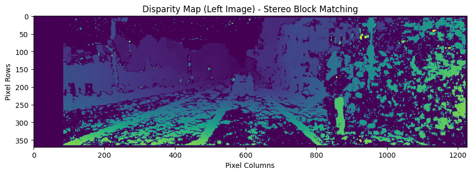
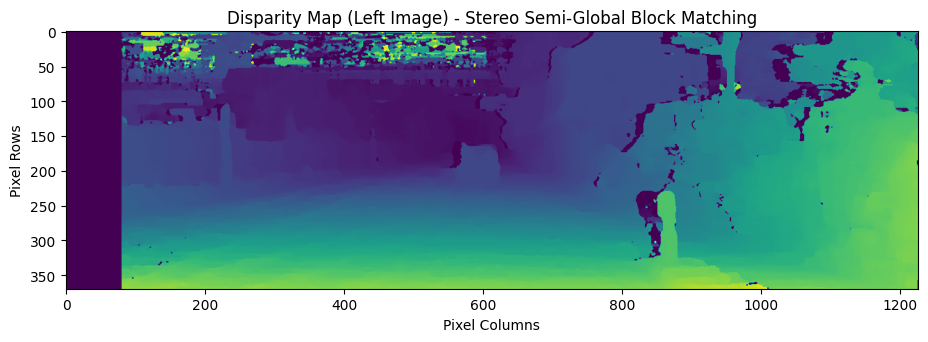
To find the necessary disparity value, we can use the stereo matching algorithms available in OpenCV, such as StereoBM or StereoSGBM. StereoBM is faster, while StereoSGBM produces better results, as we will see in practice.
By applying these equations and utilizing the appropriate stereo matching algorithm, we can estimate the depth accurately and reconstruct 3D coordinates from the stereo pair of images.
At first we define two vital parameters, “SAD window” and “block size”. In the context of stereo vision and disparity mapping, the terms “SAD window” and “block size” refer to parameters that affect the matching algorithm used to calculate disparities between corresponding points in the left and right stereo images.
- SAD Window (Sum of Absolute Differences Window): The SAD window, also known as the matching window or kernel, defines the neighborhood around a pixel in the left image that is considered for matching with the corresponding neighborhood in the right image. It represents the region within which the algorithm searches for similarities to determine the disparity.
The size of the SAD window determines the spatial extent of the matching process. A larger window size allows for capturing more context and potentially leads to more accurate disparity estimation, but it also increases computational complexity. The SAD window is usually a square or rectangular region centered around each pixel.
- Block Size: The block size specifies the dimensions of the blocks or patches within the SAD window that are compared during the matching process. It defines the size of the local regions used for computing disparities.
A larger block size means that more pixels are considered during matching, which can improve robustness against noise and texture variations. However, increasing the block size also increases the computational cost. Typically, the block size is an odd number to have a well-defined center pixel for comparison.
Both the SAD window size and block size are important parameters that influence the trade-off between accuracy and computational efficiency in stereo matching algorithms. The optimal values for these parameters depend on factors such as image resolution, scene complexity, and noise characteristics, and they may require experimentation and tuning for specific applications.
To compute the disparity map for the left image using the specified matcher we use the function below:
def compute_disp_left(img_left, img_right,sad_window,block_size, matcher_name='bm'):
    '''
    Arguments:
    img_left -- image from the left camera
    img_right -- image from the right camera

    Optional Argument:
    matcher_name -- (str) the matcher name, can be 'bm' for StereoBM or 'sgbm' for StereoSGBM matching

    Returns:
    disp_left -- disparity map for the left camera image
    '''

    # Set the parameters for disparity calculation
    num_disparities = sad_window * 16
    # Convert the input images to grayscale
    img_left_gray = cv2.cvtColor(img_left, cv2.COLOR_BGR2GRAY)
    img_right_gray = cv2.cvtColor(img_right, cv2.COLOR_BGR2GRAY)

    # Create the stereo matcher based on the selected method
    if matcher_name == 'bm':
        matcher = cv2.StereoBM_create(numDisparities=num_disparities, blockSize=block_size)
    elif matcher_name == 'sgbm':
        matcher = cv2.StereoSGBM_create(
            numDisparities=num_disparities,
            minDisparity=0,
            blockSize=block_size,
            P1=8 * 3 * sad_window ** 2,
            P2=32 * 3 * sad_window ** 2,
            mode=cv2.STEREO_SGBM_MODE_SGBM_3WAY
        )

    # Compute the disparity map
    disparity = matcher.compute(img_left_gray, img_right_gray)

    # Normalize the disparity map for visualization
    disparity_normalized = cv2.normalize(disparity, None, alpha=0, beta=255, norm_type=cv2.NORM_MINMAX, dtype=cv2.CV_8U)

    # Compute the disparity map for the left camera image and return it
    disp_left = disparity.astype(np.float32) / 16
    return disp_left
sad_window = 5
block_size = 11

disp_left = compute_disp_left(handler.first_image_left, handler.first_image_right, sad_window, block_size, matcher_name='bm')
# Set the figure size
plt.figure(figsize=(11, 7))
# Set the plot title
plt.title('Disparity Map (Left Image) - Stereo Block Matching')
# Display the disparity map
plt.imshow(disp_left)
# Add axis labels
plt.xlabel('Pixel Columns')
plt.ylabel('Pixel Rows')
# Show the plot
plt.show()

# Compute the disparity map for the left image
disp_left = compute_disp_left(handler.first_image_left, handler.first_image_right, sad_window, block_size, matcher_name='sgbm')
# Set the figure size
plt.figure(figsize=(11, 7))
# Set the plot title
plt.title('Disparity Map (Left Image) - Stereo Semi-Global Block Matching')
# Display the disparity map
plt.imshow(disp_left)
# Add axis labels
plt.xlabel('Pixel Columns')
plt.ylabel('Pixel Rows')
# Show the plot
plt.show()
StereoBM Vs. StereoSGBM
StereoBM and StereoSGBM are algorithms used in stereo vision for computing the disparity map from a pair of stereo images which are both provided by the OpenCV library and offer different approaches to stereo matching.
StereoBM (Stereo Block Matching):
- StereoBM is a block matching algorithm that operates on grayscale images.
- It works by comparing blocks of pixels between the left and right images and finding the best matching block based on a predefined matching cost.
- The disparity is then computed by calculating the difference in the horizontal pixel coordinates of the matching blocks.
- StereoBM is relatively fast and suitable for real-time applications but may not handle challenging scenes with textureless or occluded regions as effectively.
StereoSGBM (Stereo Semi-Global Block Matching):
- StereoSGBM is an extension of the StereoBM algorithm that addresses some of its limitations.
- It incorporates additional steps such as semi-global optimization to refine the disparity map and handle occlusions and textureless regions more robustly.
- StereoSGBM also considers a wider range of disparities during the matching process, allowing for more accurate depth estimation.
- It takes into account various cost factors, such as the uniqueness of matches and the smoothness of disparities, to improve the overall quality of the disparity map.
- However, StereoSGBM is computationally more expensive than StereoBM due to the additional optimization steps involved.
Both StereoBM and StereoSGBM are widely used in stereo vision applications for tasks such as 3D reconstruction, depth estimation, object detection, and robot navigation. The choice between the two algorithms depends on the specific requirements of the application, including the scene complexity, computational resources available, and desired accuracy.
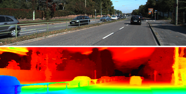
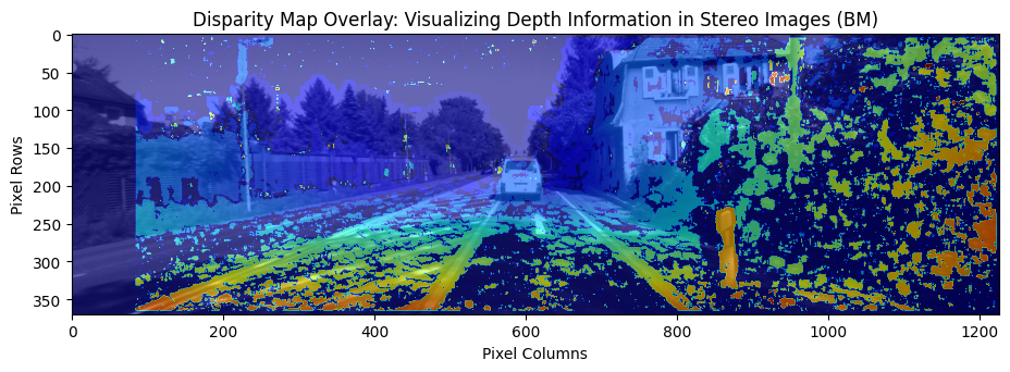
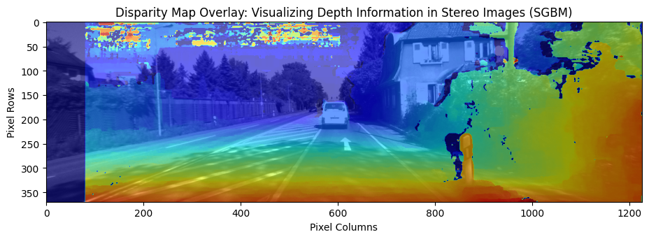
The code below is used to visualize the disparity map obtained from stereo image pairs. The disparity map contains depth information about the scene, enabling us to perceive the 3D structure of objects within the images. By overlaying the disparity map onto the main image, we can visualize the depth variations and understand the relative distances of objects in the scene. This visualization aids in applications such as depth estimation, 3D reconstruction, object detection, and scene understanding.
# Compute the disparity map
disp_left = compute_disp_left(handler.first_image_left, handler.first_image_right, sad_window, block_size, matcher_name='bm')

# Display the main image with the disparity map as overlay
plt.figure(figsize=(11, 7))
plt.title('Disparity Map Overlay: Visualizing Depth Information in Stereo Images (BM)')

plt.imshow(handler.first_image_left)
plt.imshow(disp_left, alpha=0.6, cmap='jet')
# Add axis labels
plt.xlabel('Pixel Columns')
plt.ylabel('Pixel Rows')
# Show the plot
plt.show()


# Compute the disparity map
disp_left = compute_disp_left(handler.first_image_left, handler.first_image_right, sad_window, block_size, matcher_name='sgbm')

# Display the main image with the disparity map as overlay
plt.figure(figsize=(11, 7))
plt.title('Disparity Map Overlay: Visualizing Depth Information in Stereo Images (SGBM)')

plt.imshow(handler.first_image_left)
plt.imshow(disp_left, alpha=0.6, cmap='jet')
# Add axis labels
plt.xlabel('Pixel Columns')
plt.ylabel('Pixel Rows')
# Show the plot
plt.show()
Feature Extraction
Feature extraction plays a critical role in computer vision tasks by capturing and representing distinct patterns or characteristics of images or image regions. These features serve as meaningful representations that enable higher-level analysis and interpretation of visual data. In this section, we will explore some advanced techniques for feature extraction in computer vision.
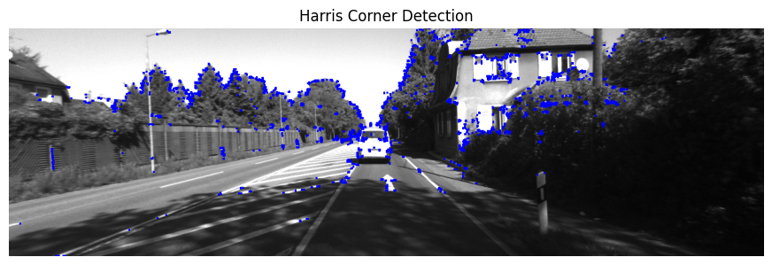
1. Harris Corner Detection
Harris Corner Detection, proposed by [Harris and Stephens] in 1988. It is a widely used algorithm for detecting corners in images. Corner points represent the junctions of two or more edges, which are highly informative for image matching and tracking. The Harris Corner Detection algorithm consists of the following steps:
Image Gradient Calculation: Compute the gradients of the image in the x and y directions using techniques such as Sobel or Prewitt operators.
Structure Tensor Computation: Based on the gradients, construct the structure tensor for each pixel. The structure tensor is a matrix that represents the local image structure at a given point.
Corner Response Function: Compute the corner response function using the structure tensor. The corner response function measures the likelihood of a pixel being a corner based on the eigenvalues of the structure tensor.
Non-maximum Suppression: Apply non-maximum suppression to the corner response function to select the most prominent corners while suppressing weaker nearby corners.
The Harris Corner Detection algorithm can be described using the following equations:
Gradient calculation: $$ \begin{equation} I_x = \frac{{\partial I}}{{\partial x}} \quad \text{and} \quad I_y = \frac{{\partial I}}{{\partial y}} \end{equation} $$
Structure tensor computation: $$ \begin{equation} M = \begin{bmatrix} I_x^2 & I_xI_y \ I_xI_y & I_y^2 \end{bmatrix} \end{equation} $$
Corner response function: $$ \begin{equation} R = \text{det}(M) - k \cdot \text{trace}(M)^2 \end{equation} $$
Non-maximum suppression:
- Select local maxima of R by comparing R with a threshold and considering neighboring pixels.
where, $I_x$ and $I_y$ are image derivatives in x and y directions respectively, $det(M)=λ1λ2$ $\text{trace}(M)=λ1+λ2$, $λ1$ and $λ2$ are the eigenvalues of $M$
Harris Corner Detection is a fundamental technique in many computer vision applications, including feature matching, image alignment, and camera calibration. The detected corners serve as robust landmarks that can be used for subsequent analysis and understanding of image content.
img = handler.first_image_left
# Load the input image
Image = handler.first_image_left
# Harris Corner Detection
gray = cv2.cvtColor(Image, cv2.COLOR_BGR2GRAY)
gray = np.float32(gray)
dst = cv2.cornerHarris(gray, 2, 3, 0.04)

# Dilate the result for marking the corners
dst = cv2.dilate(dst, None)

# Create a copy of the image to display the detected corners
image = Image.copy()

# Threshold for an optimal value, it may vary depending on the image.
image[dst>0.01*dst.max()]=[0,0,255]

# Display the image with detected corners
plt.figure(figsize=(11, 6))
plt.imshow(image, cmap='gray')
plt.title('Harris Corner Detection')
plt.axis('off')
plt.show()
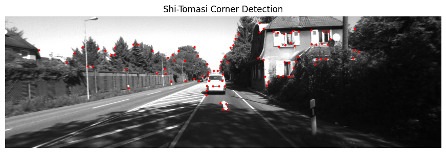
2. Shi-Tomasi Corner Detector & Good Features to Track
The Shi-Tomasi Corner Detector, also known as the [Good Features to Track] algorithm, is an improvement over the Harris Corner Detection algorithm. It provides a more robust and accurate method for detecting corners in an image. This algorithm selects the most distinctive corners based on a corner response measure. The steps involved in the Shi-Tomasi Corner Detection algorithm are as follows:
Image Gradient Calculation: Compute the gradients of the image in the x and y directions using techniques such as Sobel or Prewitt operators.
Structure Tensor Computation: Based on the gradients, construct the structure tensor for each pixel.
Eigenvalue Calculation: Compute the eigenvalues of the structure tensor for each pixel. The eigenvalues represent the principal curvatures of the local image structure.
Corner Response Calculation: Calculate the corner response measure using the eigenvalues. The corner response measure is defined as the minimum eigenvalue or a combination of the eigenvalues.
Non-maximum Suppression: Apply non-maximum suppression to select the most significant corners while suppressing weaker nearby corners.
The Shi-Tomasi Corner Detector algorithm can be described using the following equations:
Gradient calculation: $$ \begin{equation} I_x = \frac{{\partial I}}{{\partial x}} \quad \text{and} \quad I_y = \frac{{\partial I}}{{\partial y}} \end{equation} $$
Structure tensor computation: $$ \begin{equation} M = \begin{bmatrix} I_x^2 & I_xI_y \ I_xI_y & I_y^2 \end{bmatrix} \end{equation} $$
Eigenvalue calculation: $$ \begin{equation} \lambda_1, \lambda_2 = \text{eigenvalues}(M) \end{equation} $$
Corner response calculation: $$ \begin{equation} R = \min(\lambda_1, \lambda_2) \end{equation} $$
Non-maximum suppression:
- Select local maxima of R by comparing R with a threshold and considering neighboring pixels.
The Shi-Tomasi Corner Detector algorithm is widely used in feature tracking, motion estimation, and image registration tasks. It provides more accurate and reliable corner detection compared to the Harris Corner Detector.
Here’s an example code snippet for implementing the Shi-Tomasi Corner Detector using OpenCV:
import cv2
import numpy as np

# Load the input image
Image = handler.first_image_left

# Create a copy of the image to display the detected corners
image = Image.copy()

# Set the maximum number of corners to detect
max_corners = 100

# Set the quality level for corner detection
quality_level = 0.01

# Set the minimum Euclidean distance between corners
min_distance = 10

# Apply Shi-Tomasi Corner Detector
corners = cv2.goodFeaturesToTrack(gray, max_corners, quality_level, min_distance)

# Convert corners to integer coordinates
corners = np.int0(corners)

# Draw detected corners on the image
for corner in corners:
    x, y = corner.ravel()
    cv2.circle(image, (x, y), 3, 255, -1)

# Display the image with detected corners using matplotlib
plt.figure(figsize=(11, 6))
plt.imshow(image, cmap='gray')
plt.title('Shi-Tomasi Corner Detection')
plt.axis('off')
plt.show()
In this code, we use the cv2.goodFeaturesToTrack() function in OpenCV to apply the Shi-Tomasi Corner Detector. It takes the image, maximum number of corners, quality level, and minimum distance as parameters. The function returns the detected corners as a NumPy array. We then convert the corners to integers and draw them on the image using circles. Finally, we display the image with the detected corners.
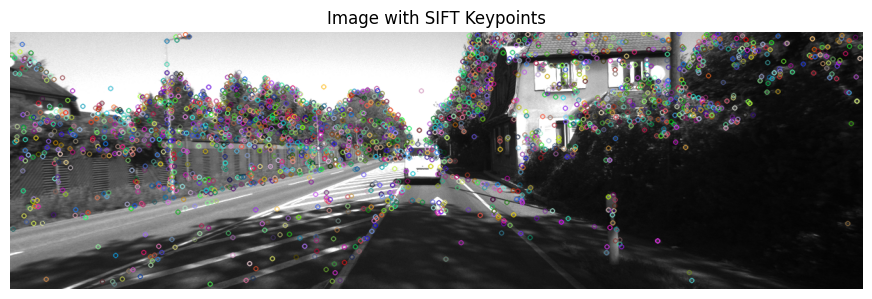
3. Scale-Invariant Feature Transform (SIFT)
The Scale-Invariant Feature Transform (SIFT) algorithm, introduced by [Lowe] in 2004, which extract keypoints and compute its descriptors. SIFT provides robustness to changes in scale, rotation, and affine transformations, making it highly effective in various real-world scenarios.
The SIFT algorithm consists of the following main steps:
Scale-space Extrema Detection: SIFT applies a Difference of Gaussian (DoG) algorithm to detect potential keypoints in different scales and locations. The DoG is obtained by subtracting blurred versions of an image at multiple scales.
Keypoint Localization: Keypoints are refined by eliminating low-contrast and poorly localized points based on the local extrema in the DoG scale space.
Orientation Assignment: Each keypoint is assigned a dominant orientation based on local image gradients. This orientation provides invariance to image rotation.
Descriptor Generation: SIFT computes a descriptor for each keypoint by considering the local image gradients and orientations. The descriptor captures the distinctive local image properties.
Keypoint Matching: Once the descriptors are computed for keypoints in multiple images, a matching algorithm is used to find corresponding keypoints between the images. This step allows for tasks such as image alignment, object tracking, and image stitching.
The SIFT algorithm incorporates several mathematical techniques to achieve scale invariance, robustness to noise, and distinctive feature representation. Some of the key equations and techniques used in SIFT are:
Difference of Gaussian (DoG): $$ \begin{equation} D(x, y, \sigma) = (G(x, y, k\sigma) - G(x, y, \sigma)) \ast I(x, y) \end{equation} $$
Gaussian function: $$ \begin{equation} G(x, y, \sigma) = \frac{1}{{2\pi\sigma^2}} \exp\left(-\frac{{x^2 + y^2}}{{2\sigma^2}}\right) \end{equation} $$
Keypoint orientation assignment: $$ \begin{equation} \theta = \text{atan2}(M_y, M_x) \end{equation} $$
Descriptor generation:
- Divide the region around the keypoint into sub-regions.
- Compute gradient magnitude and orientation for each pixel in each sub-region.
- Construct a histogram of gradient orientations in each sub-region.
- Concatenate the histograms to form the final descriptor.
# Load the input image
Image = handler.first_image_left
# Create a copy of the image
image = Image.copy()
# Create SIFT object
sift = cv2.SIFT_create()

# Detect keypoints and compute descriptors
keypoints, descriptors = sift.detectAndCompute(image, None)

# Draw keypoints on the image
image_with_keypoints = cv2.drawKeypoints(image, keypoints, None)
image = cv2.cvtColor(image_with_keypoints, cv2.COLOR_BGR2RGB)
# Display the image with keypoints using matplotlib
plt.figure(figsize=(11, 6))
plt.imshow(image)
plt.title('Image with SIFT Keypoints')
plt.axis('off')
plt.show()
4. Speeded-Up Robust Features (SURF)
The [Speeded-Up Robust Features (SURF)] algorithm, introduced by Bay et al. in 2006, provides an efficient alternative to SIFT. SURF extracts robust and distinctive features while achieving faster computation. The main steps of SURF are as follows:
Scale-space Extrema Detection: SURF applies a Hessian matrix-based approach to detect keypoints at multiple scales. The determinant of the Hessian matrix is used to identify potential interest points.
Orientation Assignment: Similar to SIFT, SURF assigns a dominant orientation to each keypoint using the sum of Haar wavelet responses.
Descriptor Generation: SURF computes a descriptor based on the distribution of Haar wavelet responses in the neighborhood of each keypoint. The wavelet responses capture the local image properties.
The SURF algorithm involves the following equations:
Hessian matrix: $$ \begin{equation} H(x, y, \sigma) = \begin{bmatrix} L_{xx}(x, y, \sigma) & L_{xy}(x, y, \sigma) \ L_{xy}(x, y, \sigma) & L_{yy}(x, y, \sigma) \end{bmatrix} \end{equation} $$
Determinant of the Hessian matrix: $$ \begin{equation}\text{Det}(H(x, y, \sigma)) = L_{xx}(x, y, \sigma) \cdot L_{yy}(x, y, \sigma) - (L_{xy}(x, y, \sigma))^2 \end{equation} $$
Keypoint orientation assignment: $$ \begin{equation}\theta = \text{atan2}\left(\sum w \cdot M_y, \sum w \cdot M_x\right) \end{equation} $$
Descriptor generation:
- Divide the region around the keypoint into sub-regions.
- Compute Haar wavelet responses in each sub-region.
- Construct a descriptor by combining and normalizing the wavelet responses.
These advanced feature extraction techniques, SIFT and SURF, offer powerful capabilities for identifying distinctive image features invariant to various transformations. They form the foundation for many computer vision applications, including object recognition, image stitching, and 3D reconstruction.
Since the SURF algorithm is not available in the current version of OpenCV, you can not use it.
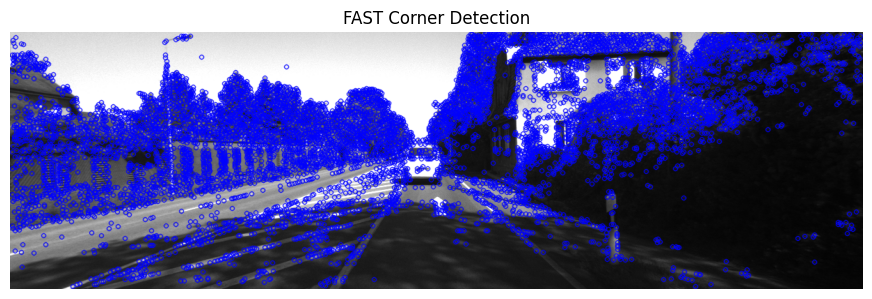
5. FAST Algorithm for Corner Detection
The [FAST (Features from Accelerated Segment Test)] algorithm is a popular corner detection method known for its efficiency and effectiveness. It aims to identify corners in images by comparing the intensity of pixels in a circular neighborhood around each pixel. The FAST algorithm is widely used in computer vision applications such as tracking, image registration, and 3D reconstruction.
The key steps involved in the FAST algorithm are as follows:
Feature Point Selection: The algorithm selects a pixel in the image as a potential corner point.
Feature Point Classification: A circular neighborhood of 16 pixels is examined around the selected point. Based on the intensities of these pixels, the algorithm classifies the selected point as a corner or not.
Non-Maximum Suppression: If the selected point is classified as a corner, non-maximum suppression is applied to remove neighboring points that have similar intensities.
The FAST algorithm utilizes a score-based approach for corner classification. It compares the intensity of the selected pixel with the intensities of the surrounding pixels to determine whether it is a corner or not. The algorithm employs a threshold value that determines the minimum intensity difference required for a pixel to be classified as a corner.
The corner detection process in the FAST algorithm involves several computations and comparisons to achieve efficiency and accuracy. The key equations and techniques used in the FAST algorithm are as follows:
Segment Test: The algorithm performs a binary test by comparing the intensities of a selected pixel with a threshold value. If the pixel’s intensity is greater or smaller than the threshold value by a certain amount, it is considered as a candidate for a corner.
Corner Classification: The algorithm compares the segment test results of neighboring pixels to classify the selected pixel as a corner. If a contiguous set of pixels in a circle satisfies the segment test criteria, the selected pixel is classified as a corner.
Non-Maximum Suppression: After identifying potential corner points, non-maximum suppression is applied to select the most salient corners. This process eliminates neighboring corners that have similar intensities, retaining only the most distinctive corners.
Here’s an example code snippet demonstrating the FAST algorithm using Python and the matplotlib library for visualization:
# Load the input image
Image = handler.first_image_left
# Create a copy of the image
image = Image.copy()

# Create FAST object
fast = cv2.FastFeatureDetector_create()

# Detect keypoints
keypoints = fast.detect(image, None)

# Draw keypoints on the image
image_with_keypoints = cv2.drawKeypoints(image, keypoints, None, color=(255, 0, 0))

# Display the image with keypoints using matplotlib
plt.figure(figsize=(11, 6))
plt.imshow(cv2.cvtColor(image_with_keypoints, cv2.COLOR_BGR2RGB))
plt.title('FAST Corner Detection')
plt.axis('off')
plt.show()
In this code, we first load the image and create a FAST object using cv2.FastFeatureDetector_create(). We then use the detect() function to detect keypoints in the image. Finally, we draw the keypoints on the image using cv2.drawKeypoints() and display the result using plt.imshow().
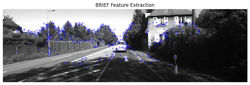
6. BRIEF (Binary Robust Independent Elementary Features)
[BRIEF (Binary Robust Independent Elementary Features)] generates a binary feature descriptor that encodes the local image properties around key points. These descriptors are efficient to compute and compare, making them suitable for real-time applications.
The BRIEF algorithm consists of the following steps:
Keypoint Selection: BRIEF selects key points in the image using a corner detection algorithm such as Harris Corner Detection or FAST Algorithm.
Descriptor Construction: For each key point, BRIEF constructs a binary feature descriptor by comparing pairs of pixel intensities in a predefined pattern around the key point.
Descriptor Matching: The binary feature descriptors are compared using a matching algorithm such as Hamming distance or Euclidean distance to find correspondences between keypoints in different images.
The BRIEF algorithm employs a pre-defined sampling pattern to select pairs of pixels around each key point. These pixel pairs are then compared, and the results are encoded into a binary string, forming the feature descriptor.
Here are the key equations and techniques used in the BRIEF algorithm:
Sampling Pattern: BRIEF uses a pre-defined sampling pattern to select pairs of pixels around each key point. The pattern specifies the pixel locations relative to the key point where the intensity comparisons will be made.
Intensity Comparison: BRIEF compares the pixel intensities at the selected pairs of locations using a simple binary test. For example, the algorithm may compare whether the intensity of the first pixel is greater than the intensity of the second pixel.
Encoding: The results of the intensity comparisons are encoded into a binary string to form the feature descriptor. Each bit in the string represents the outcome of a particular intensity comparison.
Descriptor Matching: BRIEF uses a distance metric, such as Hamming distance or Euclidean distance, to compare the binary feature descriptors of keypoints in different images. The distance measure determines the similarity between descriptors and helps in matching keypoints.
Here’s an example code snippet demonstrating the BRIEF algorithm using Python and the matplotlib library for visualization:
# Load the input image
Image = handler.first_image_left
# Create a copy of the image
image = Image.copy()

# Initiate FAST detector
star = cv2.xfeatures2d.StarDetector_create()
# Initiate BRIEF extractor
brief = cv2.xfeatures2d.BriefDescriptorExtractor_create()
# find the keypoints with STAR
kp = star.detect(image,None)
# compute the descriptors with BRIEF
kp, des = brief.compute(image, kp)

# Draw keypoints on the image
image_with_keypoints = cv2.drawKeypoints(image, kp, None, color=(255, 0, 0))

# Display the image with keypoints using matplotlib
plt.figure(figsize=(11, 6))
plt.imshow(cv2.cvtColor(image_with_keypoints, cv2.COLOR_BGR2RGB))
plt.title('BRIEF Feature Extraction')
plt.axis('off')
plt.show()
In this code, we first load the image and create a BRIEF object using cv2.xfeatures2d.BriefDescriptorExtractor_create(). We then use the detect() function to detect keypoints in the image and compute the BRIEF descriptors using brief.compute(). Finally, we draw the keypoints on the image using cv2.drawKeypoints() and display the result using plt.imshow().
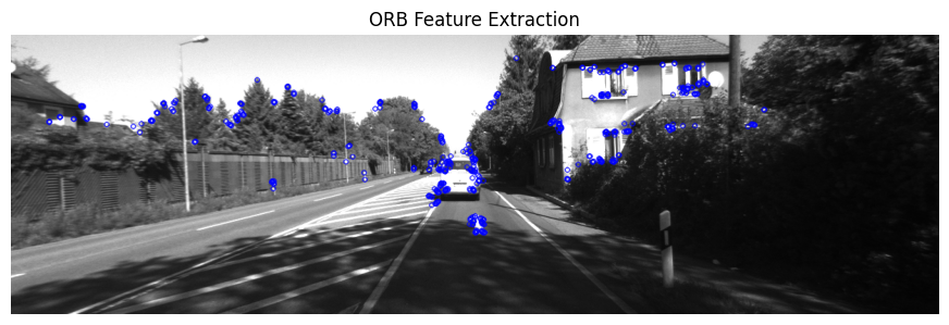
ORB (Oriented FAST and Rotated BRIEF)
[ORB (Oriented FAST and Rotated BRIEF)] combines the efficiency of the FAST corner detector with the robustness of the BRIEF descriptor. It introduces modifications to both the corner detection and descriptor computation steps to improve the performance and robustness of feature extraction.
The ORB algorithm consists of the following steps:
Keypoint Detection: ORB detects keypoints in the image using the FAST corner detection algorithm. FAST efficiently identifies corner-like features based on intensity variations in a circular neighborhood.
Orientation Assignment: ORB assigns an orientation to each keypoint to make the feature descriptor rotation-invariant. It computes a dominant orientation based on the intensity distribution in the region surrounding the keypoint.
Descriptor Construction: ORB constructs a binary feature descriptor by comparing pairs of pixel intensities in a predefined pattern around the keypoint. The BRIEF descriptor is modified to account for the assigned orientation, making it rotation-invariant.
Descriptor Matching: The binary feature descriptors of keypoints in different images are compared using a distance metric such as Hamming distance or Euclidean distance to establish correspondences between keypoints.
The ORB algorithm incorporates several optimizations and modifications to enhance its performance, including efficient sampling, orientation estimation, and scale pyramid representation.
Here are the key equations and techniques used in the ORB algorithm:
FAST Corner Detection: The FAST algorithm compares the intensity of pixels in a circular neighborhood around each pixel to identify corners. It employs a threshold and requires a sufficient number of contiguous pixels to be brighter or darker than the central pixel for it to be considered a corner.
BRIEF Descriptor: ORB uses a binary descriptor similar to BRIEF, which compares pairs of pixel intensities. However, ORB modifies BRIEF to account for the assigned orientation of keypoints. This modification involves rotating the sampling pattern according to the keypoint orientation.
Orientation Assignment: ORB assigns an orientation to each keypoint by estimating the dominant direction of intensity variations around the keypoint. It calculates the intensity centroid and computes the principal orientation using the moments of the intensity distribution.
Descriptor Matching: ORB compares the binary feature descriptors of keypoints using a distance metric such as Hamming distance or Euclidean distance. The distance measure determines the similarity between descriptors and aids in matching keypoints.
Here’s an example code snippet demonstrating the ORB algorithm using Python and the matplotlib library for visualization:
# Load the input image
Image = handler.first_image_left
# Create a copy of the image
image = Image.copy()

# Create ORB object
orb = cv2.ORB_create()

# Detect keypoints
keypoints = orb.detect(image, None)

# Compute ORB descriptors
keypoints, descriptors = orb.compute(image, keypoints)

# Draw keypoints on the image
image_with_keypoints = cv2.drawKeypoints(image, keypoints, None, color=(255, 0, 0))

# Display the image with keypoints using matplotlib
plt.figure(figsize=(11, 6))
plt.imshow(cv2.cvtColor(image_with_keypoints, cv2.COLOR_BGR2RGB))
plt.title('ORB Feature Extraction')
plt.axis('off')
plt.show()
In this code, we first load the image and create an ORB object using cv2.ORB_create(). We then use the detect() function to detect keypoints in the image and compute the ORB descriptors using orb.compute(). Finally, we draw the keypoints on the image
using cv2.drawKeypoints() and display the result using plt.imshow().
Feature Matching
Feature matching is a fundamental task in computer vision that aims to establish correspondences between features in different images or frames. It plays a crucial role in various applications such as image alignment, object recognition, motion tracking, and 3D reconstruction. The goal is to identify corresponding features across different images or frames, which enables us to understand the spatial relationships and transformations between them.
Descriptor Distance Measures
Descriptor distance measures play a vital role in feature matching by quantifying the similarity or dissimilarity between feature descriptors. These measures help determine the quality and accuracy of matches. Here, we will discuss three commonly used descriptor distance measures:
Euclidean Distance: The Euclidean distance is a fundamental distance measure used in many feature matching algorithms. It calculates the straight-line distance between two feature descriptors in the descriptor space. Mathematically, the Euclidean distance between two descriptors $x$ and $y$ with $N$ dimensions can be expressed as:
$$\begin{equation}d(x, y) = \sqrt{\sum_{i=1}^{N}(x_i - y_i)^2} \end{equation}$$
The Euclidean distance is suitable for continuous-valued feature descriptors.
Hamming Distance: The Hamming distance is specifically used for binary feature descriptors, where each bit represents a certain feature characteristic. It measures the number of differing bits between two binary strings. For example, it is commonly used with binary descriptors like BRIEF or ORB. Mathematically, the Hamming distance between two binary descriptors $x$ and $y$ with $N$ bits can be calculated as:
$$\begin{equation}d(x, y) = \sum_{i=1}^{N}(x_i \oplus y_i) \end{equation}$$
Here, $x_i$ and $y_i$ represent the bits of the binary strings $x$ and $y$, respectively, and $\oplus$ denotes the XOR operation.
Cosine Similarity: Cosine similarity is often employed in high-dimensional feature spaces. It measures the cosine of the angle between two feature vectors in the descriptor space, providing a similarity measure rather than a distance measure. Mathematically, the cosine similarity between two feature vectors $x$ and $y$ can be computed as:
$$\begin{equation}\text{similarity}(x, y) = \frac{x \cdot y}{|x| \cdot |y|} \end{equation}$$
Here, $x \cdot y$ represents the dot product of $x$ and $y$, and $$|x|$ and $|y|$ denote the Euclidean norms of $x$ and $y$, respectively.
Matching Techniques
Matching techniques aim to establish correspondences between feature descriptors, enabling the identification of similar features in different images or frames. Below, we discuss three common matching techniques:
Brute-Force Matching: Brute-force matching is a straightforward approach where each feature in one image is compared with all the features in the other image using a chosen distance measure. The best match is determined based on the minimum distance or maximum similarity score. Brute-force matching exhaustively searches for the most similar features, ensuring the best match. However, it can be computationally expensive for large-scale matching tasks.
FLANN (Fast Library for Approximate Nearest Neighbors) Matching: FLANN is an efficient algorithm for approximate nearest neighbor search. It constructs an index structure, such as a kd-tree or an approximate k-means tree, to enable fast retrieval of approximate nearest neighbors. FLANN is particularly useful in high-dimensional feature spaces where the computational cost of exact matching methods, such as brute-force matching, becomes prohibitive. By providing approximate matches, FLANN significantly reduces the time required for matching.
Ratio Test: The ratio test is a post-processing step commonly applied to feature matching to filter out ambiguous matches and enhance matching accuracy. It involves comparing the distance to the best match with the distance to the second-best match. If the ratio between these distances is below a specified threshold, the match is considered valid. By setting a threshold,
the ratio test ensures that matches are distinctive and significantly better than alternative matches. This test helps reduce false positives and improves the robustness of feature matching.
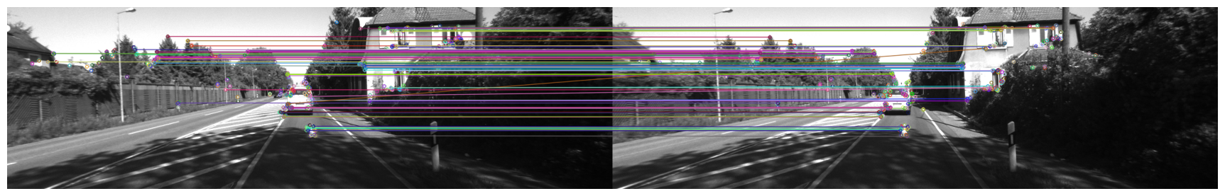
Code Example: Feature Matching with Brute-Force Matching and Euclidean Distance
Here is an example code snippet that demonstrates feature matching using the brute-force matching technique with Euclidean distance as the descriptor distance measure:
image1 = handler.first_image_left
image2 = handler.first_image_right

# Create feature detector and descriptor extractor
detector = cv2.ORB_create()
descriptor = cv2.ORB_create()

# Detect and compute keypoints and descriptors for both images
keypoints1, descriptors1 = detector.detectAndCompute(image1, None)
keypoints2, descriptors2 = detector.detectAndCompute(image2, None)

# Create a brute-force matcher with Euclidean distance
matcher = cv2.BFMatcher(cv2.NORM_L2)

# Perform matching
matches = matcher.match(descriptors1, descriptors2)

# Sort matches by distance
matches = sorted(matches, key=lambda x: x.distance)

# Draw top N matches
N = 10
matched_image = cv2.drawMatches(image1, keypoints1, image2, keypoints2, matches[:N], None)

# Convert the image to RGB format for display
matched_image_rgb = cv2.cvtColor(matched_image, cv2.COLOR_BGR2RGB)

# Display the matched image using matplotlib
plt.figure(figsize=(22, 8))
plt.imshow(matched_image_rgb)
plt.axis('off')
plt.show()
In this code example, we use the ORB feature detector and descriptor extractor to detect keypoints and compute descriptors for both images. Then, a brute-force matcher with Euclidean distance is created to perform matching on the descriptors. The matches are sorted based on distance, and the top N matches are visualized using cv2.drawMatches(). Finally, the matched image is displayed using plt.imshow().
Note: Make sure to replace 'image1.jpg' and 'image2.jpg' with the paths to your own image files.
This feature matching code demonstrates one possible implementation using the brute-force matching technique with Euclidean distance. It can be customized by selecting different distance measures, employing alternative matching techniques like FLANN, or adjusting parameters such as the ratio threshold in the ratio test to suit specific requirements and achieve optimal matching results.
[ Click hear to see full screed ]
Point Cloud to Image Projection
Point cloud to image projection is a crucial step in 3D reconstruction and visualization tasks. It involves mapping the points in a 3D point cloud onto a 2D image plane to generate a corresponding image representation. This projection allows us to visualize the 3D scene from different viewpoints or perspectives. Here, we discuss the process of projecting a point cloud onto an image plane.
Given a point cloud composed of 3D points $P_i = (X_i, Y_i, Z_i)$ and an intrinsic camera matrix $\mathbf{K}$, the projection of a 3D point onto a 2D image plane can be computed using the following steps:
Homogeneous Coordinate Transformation: The 3D point $P_i$ is represented in homogeneous coordinates as $\mathbf{P}_i = (X_i, Y_i, Z_i, 1)$. Homogeneous coordinates allow us to perform transformations using matrix operations.
World to Camera Transformation: The point $\mathbf{P}_i$ is transformed from the world coordinate system to the camera coordinate system using the camera extrinsic matrix $\mathbf{E}$. The transformation can be expressed as $\mathbf{P}_i’ = \mathbf{E} \cdot \mathbf{P}_i$.
Perspective Projection: The transformed point $\mathbf{P}_i’$ in the camera coordinate system is projected onto the image plane using perspective projection. This projection accounts for the camera intrinsic parameters, such as focal length and principal point, defined by the intrinsic camera matrix $\mathbf{K}$. The projection can be computed as $\mathbf{p}_i = \mathbf{K} \cdot \mathbf{P}_i’$.
Normalization: The projected point $\mathbf{p}_i$ is normalized by dividing its $x$ and $y$ coordinates by its $z$ coordinate to obtain the 2D image coordinates. The normalized coordinates are given by $x = \frac{p_x}{p_z}$ and $y = \frac{p_y}{p_z}$.
Clipping: The projected point is checked against the image boundaries to ensure that it lies within the valid image region. Points outside the image boundaries are typically discarded or handled using appropriate techniques.
By repeating these steps for each point in the point cloud, we can project the entire point cloud onto the image plane, generating a corresponding image representation.
Code Example: Point Cloud to Image Projection
def project_point_cloud_to_image(point_cloud, image_height, image_width, transformation_matrix, projection_matrix):
    """
    Projects a point cloud onto an image plane by transforming the X, Y, Z coordinates of the points
    to the camera frame using the transformation matrix, and then projecting them using the camera's
    projection matrix.

    Arguments:
    point_cloud -- array of shape Nx4 containing (X, Y, Z, reflectivity) coordinates of the point cloud
    image_height -- height (in pixels) of the image plane
    image_width -- width (in pixels) of the image plane
    transformation_matrix -- 3x4 transformation matrix between the lidar (X, Y, Z, 1) homogeneous and camera (X, Y, Z)
                             coordinate frames
    projection_matrix -- projection matrix of the camera (should have identity transformation if the
                         transformation matrix is used)

    Returns:
    rendered_image -- a (image_height x image_width) array containing depth (Z) information from the lidar scan
    """
    # Ignore points with X values less than or equal to zero (behind the lidar)
    point_cloud = point_cloud[point_cloud[:, 0] > 0]

    # Drop the last column (reflectivity) and replace it with ones to make coordinates homogeneous
    point_cloud_homogeneous = np.hstack([point_cloud[:, :3], np.ones((point_cloud.shape[0], 1))])

    # Transform the point cloud into the camera coordinate frame
    transformed_cloud = np.dot(transformation_matrix, point_cloud_homogeneous.T).T

    # Ignore points behind the camera
    transformed_cloud = transformed_cloud[transformed_cloud[:, 2] > 0]

    # Extract the Z coordinates (depth) from the camera
    depth = transformed_cloud[:, 2].copy()

    # Project the coordinates in the camera frame onto a flat plane at Z=1 by dividing by Z
    transformed_cloud /= transformed_cloud[:, 2].reshape(-1, 1)

    # Add a row of ones to make the 3D coordinates on the plane homogeneous for dotting with the projection matrix
    transformed_cloud_homogeneous = np.vstack([transformed_cloud.T, np.ones(transformed_cloud.shape[0])])

    # Get the pixel coordinates (X, Y) in the camera coordinate frame
    projected_points = np.dot(projection_matrix, transformed_cloud_homogeneous)
    projected_points = projected_points.T

    # Round the pixel coordinates to integers for indexing
    pixel_coordinates = np.round(projected_points[:, :2]).astype('int')

    # Limit the pixel coordinates to those within the image plane boundaries
    indices = np.where((pixel_coordinates[:, 0] < image_width)
                       & (pixel_coordinates[:, 0] >= 0)
                       & (pixel_coordinates[:, 1] < image_height)
                       & (pixel_coordinates[:, 1] >= 0))
    pixel_coordinates = pixel_coordinates[indices]
    depth = depth[indices]

    # Create an empty image, then fill it with the depths of each point
    rendered_image = np.zeros((image_height, image_width))
    for j, (u, v) in enumerate(pixel_coordinates):
        if 0 <= u < image_width and 0 <= v < image_height:
            rendered_image[v, u] = depth[j]

    # Fill zero values with a large distance so they will be ignored
    rendered_image[rendered_image == 0.0] = 3861.45

    return rendered_image
In this code example, the function project_point_cloud_to_image takes a point cloud, camera extrinsic matrix, camera intrinsic matrix, image width, and image height as input parameters. It performs the steps described above to project the point cloud onto the image plane. The projected points and valid indices are returned for further processing or visualization.
Note: The actual implementation may vary depending on the library or framework used for point cloud and image processing. The provided code serves as a general guide to the projection process and may require modification to suit specific requirements and conventions.
depth_lidar = pointcloud2image(handler.first_pointcloud,
                            handler.imheight,
                            handler.imwidth,handler.Tr, handler.P0)
depth_stereo = compute_disp_left(handler.first_image_left,
                            handler.first_image_right,
                            5,11, matcher_name='bm')

fig, (ax1, ax2) = plt.subplots(2,1, figsize=(12, 8))

ax1.imshow(depth_lidar)
ax1.set_title('Lidar Depth Map')
ax1.axis('off')

ax2.imshow(depth_stereo)
ax2.set_title('Stereo Depth Map')
ax2.axis('off')

plt.tight_layout()
plt.show()
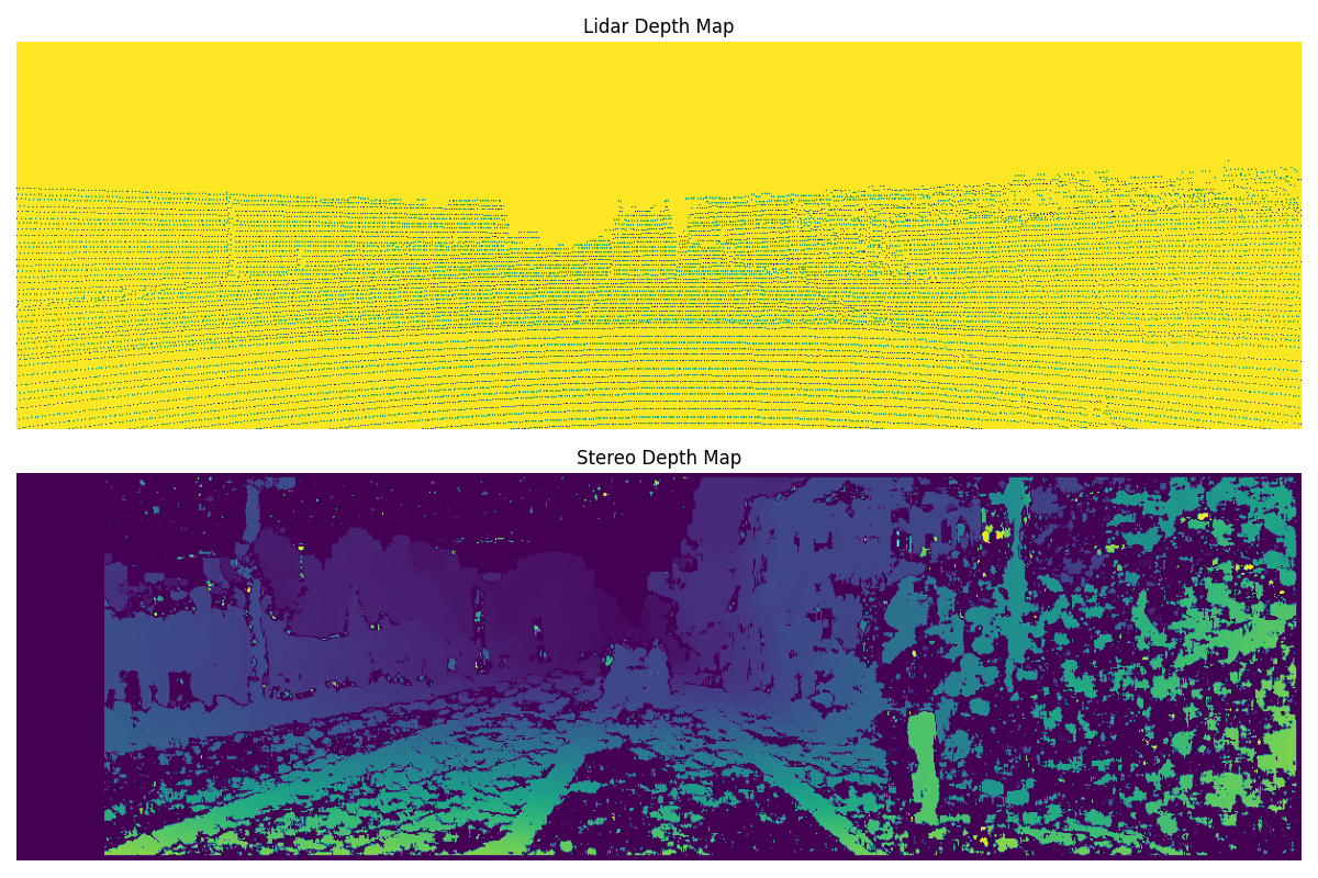
Visualizing LiDAR Pointcloud
import numpy as np
import plotly.graph_objects as go

def visualize_pointcloud(pointcloud):
    """
    Visualizes a lidar point cloud using Plotly

    Arguments:
    pointcloud  --  array of shape Nx4 containing (X, Y, Z, reflectivity)
                    coordinates of the point cloud
    """
    # Extract coordinates from the point cloud
    xs = pointcloud[:, 0]
    ys = pointcloud[:, 1]
    zs = pointcloud[:, 2]

    # Create a 3D scatter plot
    fig = go.Figure(data=[go.Scatter3d(x=xs, y=ys, z=zs, mode='markers',
                          marker=dict(size=1, color=zs,
                          colorscale='Viridis'))])

    # Set the layout options
    fig.update_layout(scene=dict(aspectmode='data',
                                 xaxis=dict(showgrid=False,
                                            showticklabels=False),
                                 yaxis=dict(showgrid=False,
                                            showticklabels=False),
                                 zaxis=dict(showgrid=False,
                                            showticklabels=False)),
                                 showlegend=False)
    # Show the plot
    fig.show()
Let’s compare the diffrence between Stereo Depth and LiDAR Depth. A comparison of depth estimation methods, specifically stereo estimation and lidar technology, offers valuable insights into the accuracy and reliability of these techniques for capturing depth information. Stereo estimation involves leveraging multiple images taken from slightly different perspectives to triangulate depth, while lidar utilizes laser beams to measure distances between the sensor and objects in its field of view. Understanding the nuances and discrepancies between these depth estimation approaches is of utmost importance in a wide range of applications, including autonomous driving, 3D mapping, and robotics.
By conducting a comparative analysis of the depth outputs obtained from stereo estimation and lidar, we can evaluate their consistency and identify potential systematic errors. The provided code allows us to filter lidar depths based on a threshold and extract corresponding depths from stereo estimation. Subsequently, the difference in depth between the two methods can be calculated and visualized through a scatter plot.
Analyzing the depth difference provides a means to assess the relative accuracy of stereo estimation and lidar. A depth difference close to zero signifies a strong agreement between the two methods, while significant deviations shed light on limitations or biases inherent to each technique. This insight is vital for comprehending the strengths and weaknesses associated with each approach and facilitates informed decision-making when choosing the most suitable method for specific applications.
By visualizing the depth difference, valuable insights can be gained regarding the particular areas or scenarios where one method excels over the other. Such analysis plays a pivotal role in driving advancements in depth sensing technologies and aids in the development of more accurate and robust systems for depth perception.
# Filter depths from lidar below a threshold
lidar_threshold = 3000
valid_depth_indices = np.where(depth_lidar < lidar_threshold)
depth_indx = np.array(list(zip(*valid_depth_indices)))

# Extract depths for comparison
stereo_depths = depth_stereo[depth_indx[:, 0], depth_indx[:, 1]]
lidar_depths = depth_lidar[depth_indx[:, 0], depth_indx[:, 1]]

# Calculate the difference between stereo depth and lidar depth
depth_difference = stereo_depths - lidar_depths

# Create scatter plot for depth difference
fig, ax = plt.subplots(figsize=(8, 6))
ax.scatter(stereo_depths, depth_difference, c='b', label='Depth Difference', alpha=0.8)
ax.axhline(0, color='r', linestyle='--')
ax.set_xlabel('Stereo Depth')
ax.set_ylabel('Depth Difference')
ax.legend()

plt.title('Difference between Stereo Depth and Lidar Depth')
plt.grid(color='gray', linestyle='--', linewidth=0.5)
plt.tight_layout()
plt.show()
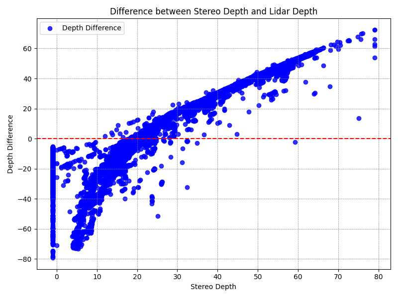
Estimate Camera Motion
Estimating camera motion is a fundamental task in computer vision and robotics, where the goal is to determine the transformation between consecutive camera frames. This transformation represents the camera’s motion in terms of rotation and translation, allowing us to understand how the camera has moved between frames. Several techniques exist to estimate camera motion, including feature-based methods and direct methods. Here, we will discuss a common feature-based method called feature point correspondence and motion estimation.
Feature Point Correspondence
Feature point correspondence is the process of identifying corresponding points between consecutive camera frames. These corresponding points serve as the basis for estimating camera motion. Commonly used feature detection algorithms such as Harris Corner Detection, Shi-Tomasi Corner Detector, or FAST Algorithm can be employed to extract feature points from each frame.
Once the feature points are detected, a technique called feature point matching is applied to find corresponding points between frames. Various matching algorithms exist, such as nearest neighbor matching and RANSAC (Random Sample Consensus). These algorithms compare the feature descriptors of each detected point to find the best matches.
Camera Motion Estimation
Once the corresponding feature points are identified, camera motion can be estimated using methods such as epipolar geometry or homography estimation.
Epipolar Geometry: Epipolar geometry is based on the geometric relationship between two camera views. Given corresponding feature points in two frames, epipolar geometry utilizes the epipolar constraint to estimate camera motion. The epipolar constraint states that the projection of a 3D point onto two camera views lies on a line called the epipolar line. By estimating the essential matrix or fundamental matrix, which encapsulates the epipolar geometry, the camera motion can be computed.
Homography Estimation: Homography estimation assumes that the camera undergoes a pure planar motion. In this case, the corresponding feature points lie on a planar surface. By estimating the homography matrix that relates the points on the plane between the frames, the camera motion can be obtained.
Camera Motion Representation
The estimated camera motion is typically represented using a transformation matrix that combines rotation and translation. There are different ways to represent camera motion, including:
- Rotation Matrix (R): A 3x3 matrix that represents the rotation component of the camera motion. It describes how the camera has rotated between frames.
- Translation Vector (t): A 3D vector that represents the translation component of the camera motion. It indicates the camera’s displacement in 3D space.
- Essential Matrix (E) or Fundamental Matrix (F): Matrices that encapsulate the geometric relationship between two camera views and encode the camera motion. They are used in epipolar geometry-based motion estimation methods.
The camera motion can be further decomposed into its individual components, such as rotation angles or Euler angles, to provide a more detailed representation of the camera’s motion.
Code Example: Camera Motion Estimation
import cv2

def estimate_camera_motion(frame1, frame2):
    # Detect feature points in frame1 and frame2
    feature_detector = cv2.FastFeatureDetector_create()
    keypoints1 = feature_detector.detect(frame1, None)
    keypoints2 = feature_detector.detect(frame2, None)

    # Extract feature descriptors
    descriptor_extractor = cv2.BRISK_create()
    _, descriptors1 = descriptor_extractor.compute(frame1, keypoints1)
    _, descriptors2 = descriptor_extractor.compute(frame2, keypoints2)

    # Match feature descriptors
    matcher = cv2.BFMatcher(cv2.NORM_HAMMING, crossCheck=True)
    matches = matcher.match(descriptors1, descriptors2)

    # Estimate camera motion
    essential_matrix, _

 = cv2.findEssentialMat(
        [kp.pt for kp in keypoints1],
        [kp.pt for kp in keypoints2],
        focal=1.0,
        pp=(0.0, 0.0),
        method=cv2.RANSAC,
        prob=0.999,
        threshold=1.0
    )
    _, rotation_matrix, translation_vector, _ = cv2.recoverPose(
        essential_matrix,
        [kp.pt for kp in keypoints1],
        [kp.pt for kp in keypoints2]
    )

    return rotation_matrix, translation_vector

# Usage
frame1 = cv2.imread('frame1.jpg')
frame2 = cv2.imread('frame2.jpg')
rotation_matrix, translation_vector = estimate_camera_motion(frame1, frame2)
In this code example, we use the OpenCV library to estimate camera motion between two frames. We detect feature points using the FAST algorithm and compute feature descriptors using the BRISK algorithm. Feature point matching is performed using the brute-force matching technique. The camera motion is estimated using the findEssentialMat and recoverPose functions, which utilize the RANSAC algorithm for robustness.
Note: The actual implementation may vary depending on the library or framework used for feature detection, descriptor extraction, and motion estimation. The provided code serves as a general guide to the process and may require modification to suit specific requirements and conventions.
Visual Odometry
Visual Odometry is a technique used in computer vision and robotics to estimate the motion of a camera by analyzing consecutive images. It plays a crucial role in applications such as autonomous navigation, simultaneous localization and mapping (SLAM), and augmented reality. Visual odometry algorithms use the information extracted from the camera images to estimate the camera’s position and orientation changes, providing valuable information for navigation and mapping tasks.
Pipeline Overview
The visual odometry pipeline typically consists of the following steps:
Feature Detection: Detect distinctive features in the image frames, such as corners or keypoints. These features serve as landmarks for tracking camera motion.
Feature Tracking: Establish correspondences between features in consecutive frames. This step ensures consistent tracking of features across frames.
Motion Estimation: Estimate the camera’s motion between frames using the tracked features. This involves computing the relative transformation (rotation and translation) between frames.
Scale Estimation: Determine the scale factor to recover the absolute scale of the camera motion. This is essential for accurate mapping and navigation.
Trajectory Estimation: Accumulate the estimated camera poses over time to compute the camera’s trajectory.
Feature-Based Visual Odometry
Feature-based visual odometry methods focus on extracting and tracking distinctive features in the images. These features can be detected using algorithms such as Harris Corner Detection, Shi-Tomasi Corner Detector, or modern deep learning-based detectors like SIFT or SURF.
Once the features are detected, they are tracked across consecutive frames. This can be achieved using techniques like optical flow, where the displacement of each feature is estimated. Alternatively, feature descriptors can be computed for each feature and matched between frames to establish correspondences.
After establishing feature correspondences, the camera’s motion can be estimated by solving the perspective-n-point (PnP) problem. The PnP problem aims to find the camera’s pose (rotation and translation) given a set of 3D points and their corresponding 2D image projections. RANSAC (Random Sample Consensus) is often used to robustly estimate the camera motion by filtering out outliers.
Once the camera motion is estimated, the scale factor can be obtained by comparing the motion of the camera to other sources of information, such as a known baseline distance or sensor data (e.g., IMU). This step is crucial for accurately reconstructing the scene and estimating the camera trajectory.
Visual Odometry Formulation
The visual odometry problem can be formulated as follows:
Given two consecutive images, denoted as (I_t) and (I_{t+1}), we aim to estimate the relative camera motion between them.
Let (P_t = {p_1, p_2, \ldots, p_n}) be the set of 3D feature points in the world coordinate system, and (p_t^i) and (p_{t+1}^i) be their corresponding 2D projections in images (I_t) and (I_{t+1}), respectively.
The goal is to estimate the camera’s pose transformation (T) from the coordinate system of (I_t) to the coordinate system of (I_{t+1}), represented as (T = (R, t)), where (R) is the rotation matrix and (t) is the translation vector.
The estimated camera motion can be represented as (T_{t \rightarrow t+1}), indicating the camera’s motion from time (t) to (t+1).
By accumulating the estimated camera motions, we can compute the camera’s trajectory over time.
Visual odometry algorithms often make assumptions such as camera motion smoothness, feature trackability, and limited scene depth variation to enhance the
estimation accuracy and robustness. Advanced techniques, such as bundle adjustment, loop closure detection, and map refinement, can also be incorporated to improve the visual odometry performance and handle challenging scenarios.
Code Example
import cv2
import numpy as np

def estimate_camera_motion(frame1, frame2):
    # Feature detection
    detector = cv2.SIFT_create()
    keypoints1, descriptors1 = detector.detectAndCompute(frame1, None)
    keypoints2, descriptors2 = detector.detectAndCompute(frame2, None)

    # Feature matching
    matcher = cv2.BFMatcher(cv2.NORM_L2)
    matches = matcher.match(descriptors1, descriptors2)

    # Extract matching keypoints
    matched_kp1 = np.array([keypoints1[m.queryIdx].pt for m in matches])
    matched_kp2 = np.array([keypoints2[m.trainIdx].pt for m in matches])

    # Estimate camera motion
    essential_matrix, mask = cv2.findEssentialMat(matched_kp1, matched_kp2, focal=1.0, pp=(0.0, 0.0))
    _, rotation_matrix, translation_vector, _ = cv2.recoverPose(essential_matrix, matched_kp1, matched_kp2)

    return rotation_matrix, translation_vector

# Usage
frame1 = cv2.imread('frame1.jpg')
frame2 = cv2.imread('frame2.jpg')
rotation_matrix, translation_vector = estimate_camera_motion(frame1, frame2)
In this code example, we use the OpenCV library to estimate the camera motion between two consecutive frames. We detect keypoints using the SIFT algorithm and compute their descriptors. Feature matching is performed using the brute-force matcher. The camera motion is estimated using the findEssentialMat and recoverPose functions, which utilize the RANSAC algorithm for robustness.
Note: The actual implementation may vary depending on the library or framework used for feature detection, descriptor extraction, and motion estimation. The provided code serves as a general guide to the process and may require modification to suit specific requirements and conventions.
You can find the Jupet-Notebook .ipynb file at github repository
References
- Geiger, Andreas, Philip Lenz, and Raquel Urtasun. “Are we ready for autonomous driving? The KITTI vision benchmark suite.” Conference on Computer Vision and Pattern Recognition (CVPR), 2012.
- KITTI Vision Benchmark Suite. http://www.cvlibs.net/datasets/kitti/
- Harris, Chris, and Mike Stephens. "A combined corner and edge detector." Alvey vision conference. Vol. 15. No. 50. 1988.
- Shi, Jianbo. "Good features to track." 1994 Proceedings of IEEE conference on computer vision and pattern recognition. IEEE, 1994.
- Lowe, David G. "Distinctive image features from scale-invariant keypoints." International journal of computer vision 60 (2004): 91-110.
- Bay, Herbert, Tinne Tuytelaars, and Luc Van Gool. "Surf: Speeded up robust features." Lecture notes in computer science 3951 (2006): 404-417.
- Rosten, Edward, and Tom Drummond. "Machine learning for high-speed corner detection." Computer Vision–ECCV 2006: 9th European Conference on Computer Vision, Graz, Austria, May 7-13, 2006. Proceedings, Part I 9. Springer Berlin Heidelberg, 2006.
- Calonder, Michael, et al. "Brief: Binary robust independent elementary features." Computer Vision–ECCV 2010: 11th European Conference on Computer Vision, Heraklion, Crete, Greece, September 5-11, 2010, Proceedings, Part IV 11. Springer Berlin Heidelberg, 2010.
- Rublee, Ethan, et al. "ORB: An efficient alternative to SIFT or SURF." 2011 International conference on computer vision. Ieee, 2011.
Arman Asgharpoor Golroudbari
Machine Learning Engineer
Machine Learning Engineer with 5+ years of experience in LLMs, transformer architectures, computer vision systems, and autonomous robotics.