RoNIN IMU Dataset
Introduction
RoNIN
The RoNIN dataset [1] contains over 40 hours of IMU sensor data from 100 human subjects with 3D ground-truth trajectories under natural human movements. This data set provides measurements of the accelerometer, gyroscope, magnetometer, and ground track, including direction and location in 327 sequences and at a frequency of 200 Hz. A two-device data collection protocol was developed. A harness was used to attach one phone to the body for 3D tracking, allowing subjects to control the other phone to collect IMU data freely. It should be noted that the ground track can only be obtained using the 3D tracker phone attached to the harness. In addition, the body trajectory is estimated instead of the IMU. RoNIN datset contians 42.7 hours of IMU-motion data over 276 sequences in 3 buildings, and collected from 100 human subjects with three Android devices. The dataset is available at Link.
How to use RoNIN dataset
The dataset can be downloaded from Here. The dataset contains following:
- Data 13.81 GB
- Pretrained_Models 57.05 MB
- seen_subjects_test_set.zip 3.15 GB
- train_dataset_1.zip 4.49 GB
- train_dataset_2.zip 3.18 GB
- unseen_subjects_test_set.zip 2.99 GB
- ronin_body_heading.zip 579.52 KB
- ronin_lstm.zip 2.29 MB
- ronin_resnet.zip 48.49 MB
- ronin_tcn.zip 5.71 MB
All HDF5 files are organized as follows
HDF5 data format
- raw:
- synced:
- pose:
- tango:
- gyro, gyro_uncalib, acce, magnet, game_rv, gravity, linacce, step, tango_pose, tango_adf_pose, rv, pressure, (optional) [wifi, gps, magnetic_rv, magnet_uncalib]
- imu:
- gyro, gyro_uncalib, acce, magnet, game_rv, gravity, linacce, step. rv, pressure, (optional) [wifi, gps, magnetic_rv, magnet_uncalib]
- time, gyro, gyro_uncalib, acce, magnet, game_rv, rv, gravity, linacce, step
- tango_pos, tango_ori, (optional) ekf_ori
Use RoNIN Dataset in Python
First, we need to import libraries
import os
import h5py
import numpy as np
import pandas as pd
import matplotlib.pyplot as plt
To access the data in each folder, a list of all folders in the directory must be created.
folder_name = prefixed = [filename for filename in os.listdir('.') if filename.startswith("a")]
Create variables to store the data
acc     = [0, 0, 0]
gyro    = [0, 0, 0]
mag     = [0, 0, 0]
ori     = [0, 0, 0, 0]
pose    = [0, 0, 0]
Import all the data files in to python
for i in range(len(folder_name)):
    load_file = folder_name[i] + '/data.hdf5'
    df = h5py.File(load_file, 'r')

    header = np.array(df.get('synced'))
    for i in range(len(np.array(df.get('synced')))):
        # np.array(df.get('synced'))[header[i]]
        if header[i] == 'acce':
            temp = np.array(df.get('synced')[header[i]])
            acc = np.vstack((acc, temp))
        if header[i] == 'gyro':
            temp = np.array(df.get('synced')[header[i]])
            gyro = np.vstack((gyro, temp))
        if header[i] == 'magnet':
            temp = np.array(df.get('synced')[header[i]])
            mag = np.vstack((mag, temp))
    header = np.array(df.get('pose'))
    for i in range(len(np.array(df.get('pose')))):
        if header[i] == 'ekf_ori':
            temp = np.array(df.get('pose')[header[i]])
            ori = np.vstack((ori, temp))
        if header[i] == 'tango_pos':
            temp = np.array(df.get('pose')[header[i]])
            pose = np.vstack((pose, temp))
At last, each variable could use to train or evaluate a deep learning model or just save in a CSV format similar to follows
df_imu = pd.DataFrame({'Acc x': acc[1:, 0], 'Acc y': acc[1:, 1], 'Acc z': acc[1:, 2], 'Gyro x': gyro[1:, 0],
                      'Gyro y': gyro[1:, 1], 'Gyro z': gyro[1:, 2], 'Mag x': mag[1:, 0], 'Mag y': mag[1:, 1], 'Mag z': mag[1:, 2]})
df_imu.to_csv('RoNIN_IMU.csv', index=False)
df_gt = pd.DataFrame({'Ori w': ori[1:, 0], 'Ori x': ori[1:, 1], 'Ori y': ori[1:, 2],
                     'Ori z': ori[1:, 3], 'Pose x': pose[1:, 0], 'Pose y': pose[1:, 1], 'Pose z': pose[1:, 2]})
df_gt.to_csv('RoNIN_GT.csv', index=False)
Also, the data could be plot by
fs = 200
dt = 1/fs
t = np.arange(0,acce.shape[0]/fs,dt)
# Plot the IMU readings
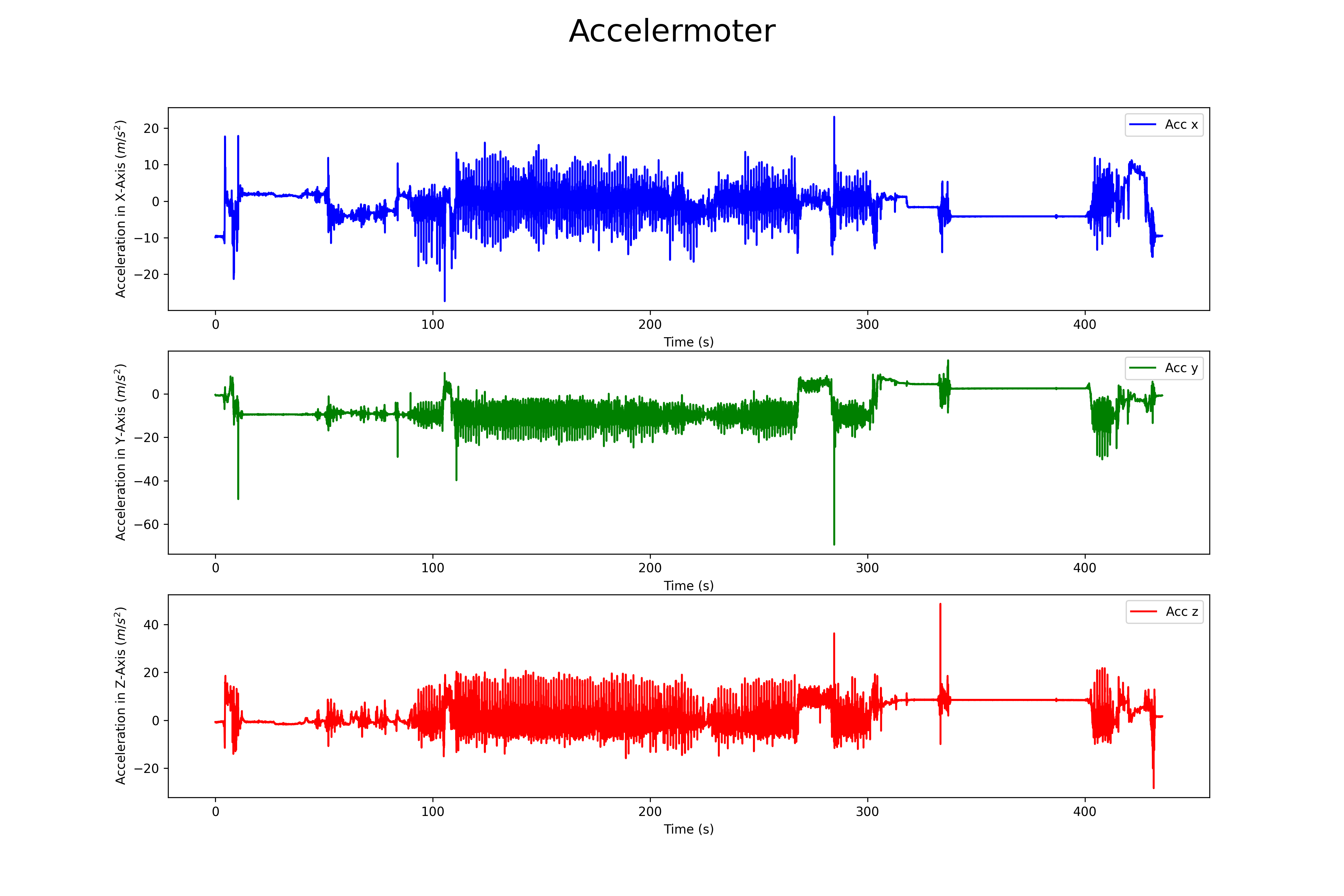
## Accelermoter
plt.figure(figsize=(15, 10))
plt.title("Accelermoter")
plt.subplot(3, 1, 1)
plt.plot(t, acc[1:, 0], label='Acc x', color='b')
plt.legend(loc="upper right")
plt.xlabel('Time (s)')
plt.ylabel('Acceleration in X-Axis ($m/s^2$)')
plt.subplot(3, 1, 2)
plt.plot(t, acc[1:, 1], label='Acc y', color='g')
plt.legend(loc="upper right")
plt.xlabel('Time (s)')
plt.ylabel('Acceleration in Y-Axis ($m/s^2$)')
plt.subplot(3, 1, 3)
plt.plot(t, acc[1:, 2], label='Acc z', color='r')
plt.xlabel('Time (s)')
plt.ylabel('Acceleration in Z-Axis ($m/s^2$)')
plt.legend(loc="upper right")
plt.suptitle("Accelermoter", fontsize=25)
plt.savefig('RoNIN_Acc.png', dpi=300)
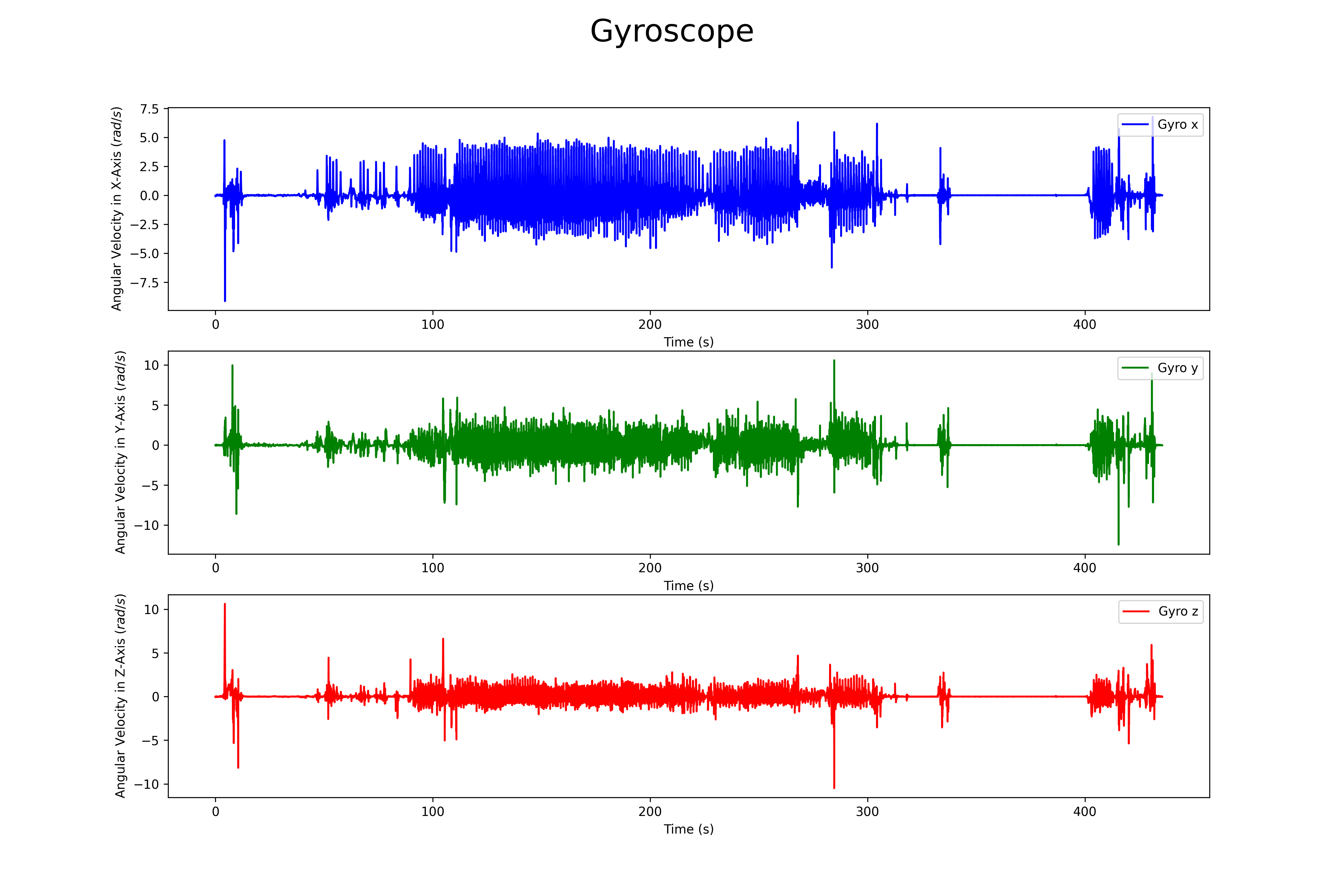
## Gyroscope
# Plotting the three axis of the gyroscope in one figure.
plt.figure(figsize=(15, 10))
plt.subplot(3, 1, 1)
plt.plot(t, gyro[1:, 0], label='Gyro x', color='b')
plt.legend(loc="upper right")
plt.xlabel('Time (s)')
plt.ylabel('Angular Velocity in X-Axis ($rad/s$)')
plt.subplot(3, 1, 2)
plt.plot(t, gyro[1:, 1], label='Gyro y', color='g')
plt.legend(loc="upper right")
plt.xlabel('Time (s)')
plt.ylabel('Angular Velocity in Y-Axis ($rad/s$)')
plt.subplot(3, 1, 3)
plt.plot(t, gyro[1:, 2], label='Gyro z', color='r')
plt.xlabel('Time (s)')
plt.ylabel('Angular Velocity in Z-Axis ($rad/s$)')
plt.legend(loc="upper right")
plt.suptitle("Gyroscope", fontsize=25)
plt.savefig('RoNIN_Gyro.png', dpi=300)
## Magnetometer
# Plotting the three axis of the magnetometer in one figure.
plt.figure(figsize=(15, 10))
plt.subplot(3, 1, 1)
plt.plot(t, mag[1:, 0], label='Mag x', color='b')
plt.legend(loc="upper right")
plt.xlabel('Time (s)')
plt.ylabel('Magnetic Field in X-Axis ($\mu T$)')
plt.subplot(3, 1, 2)
plt.plot(t, mag[1:, 1], label='Mag y', color='g')
plt.legend(loc="upper right")
plt.xlabel('Time (s)')
plt.ylabel('Magnetic Field in Y-Axis ($\mu T$)')
plt.subplot(3, 1, 3)
plt.plot(t, mag[1:, 2], label='Mag z', color='r')
plt.xlabel('Time (s)')
plt.ylabel('Magnetic Field in Z-Axis ($\mu T$)')
plt.legend(loc="upper right")
plt.suptitle("Magnetometer", fontsize=25)
plt.savefig('RoNIN_Mag.png', dpi=300)
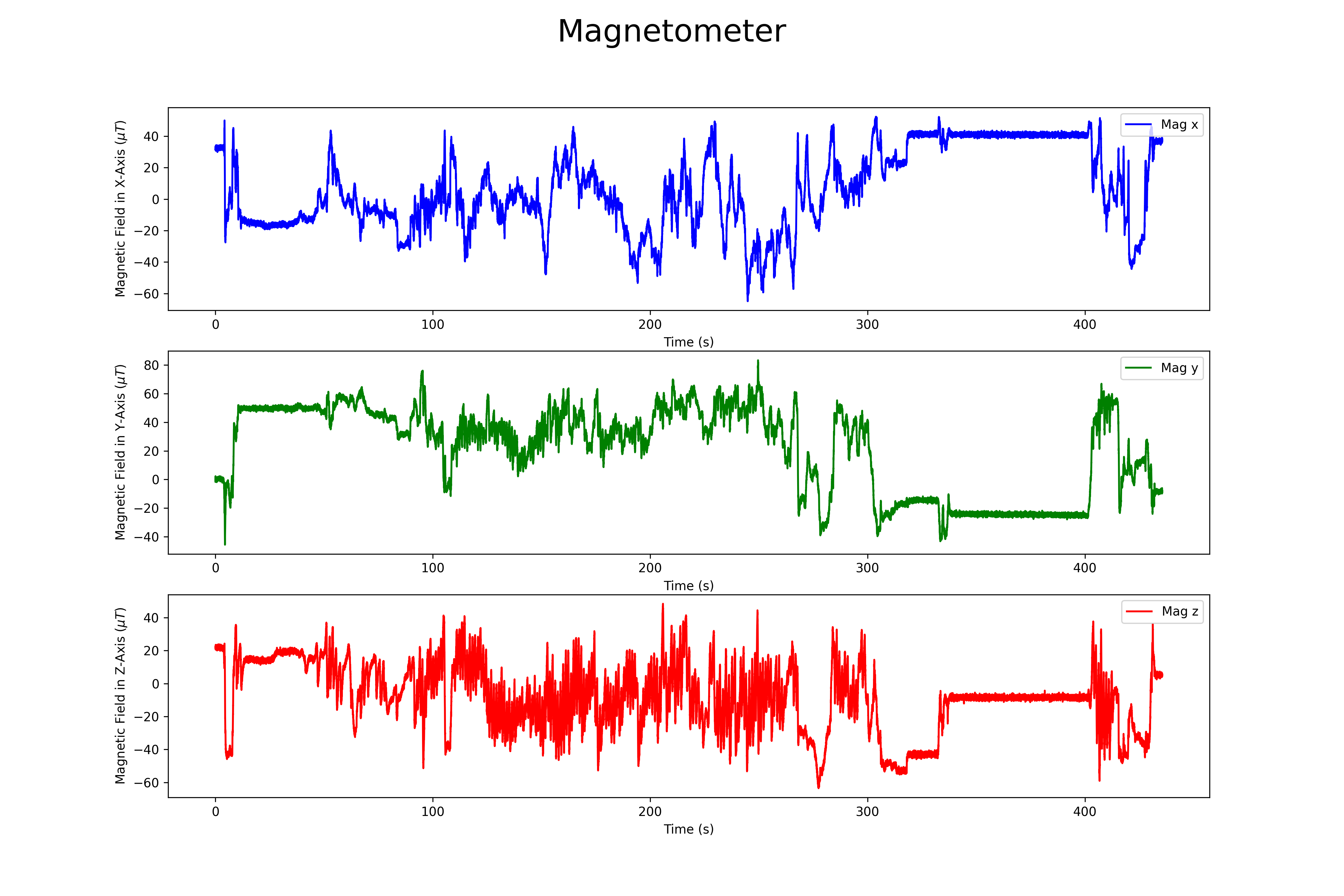
The magnetomer 3d scatter plot can be found here

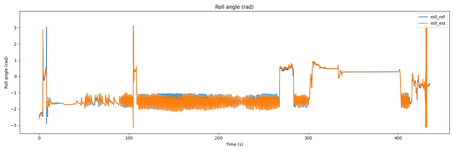
To test the dataset, we can use AHRS [2] library which has multiple sensor fusion algorithm for python. The Madgwick algorithm has been chosen as SFA.
fs = 200
dt = 1/fs
t = np.arange(0, acc.shape[0]/fs, dt)
madgwick = sfa.Madgwick(gyr=gyro, acc=acc, mag=mag, frequency=fs)
roll_ref, pitch_ref, yaw_ref = quat2eul(ori)
roll_est, pitch_est, yaw_est = quat2eul(madgwick.Q)
# Plot the results
# Roll
plt.figure(figsize=(15, 5))
plt.plot(t, roll_ref, label='roll_ref')
plt.plot(t, roll_est, label='roll_est')
plt.title('Roll angle (rad)')
plt.xlabel('Time (s)')
plt.ylabel('Roll angle (rad)')
plt.ylim(-3.5, 3.999)
plt.legend(loc='upper right')
plt.show()
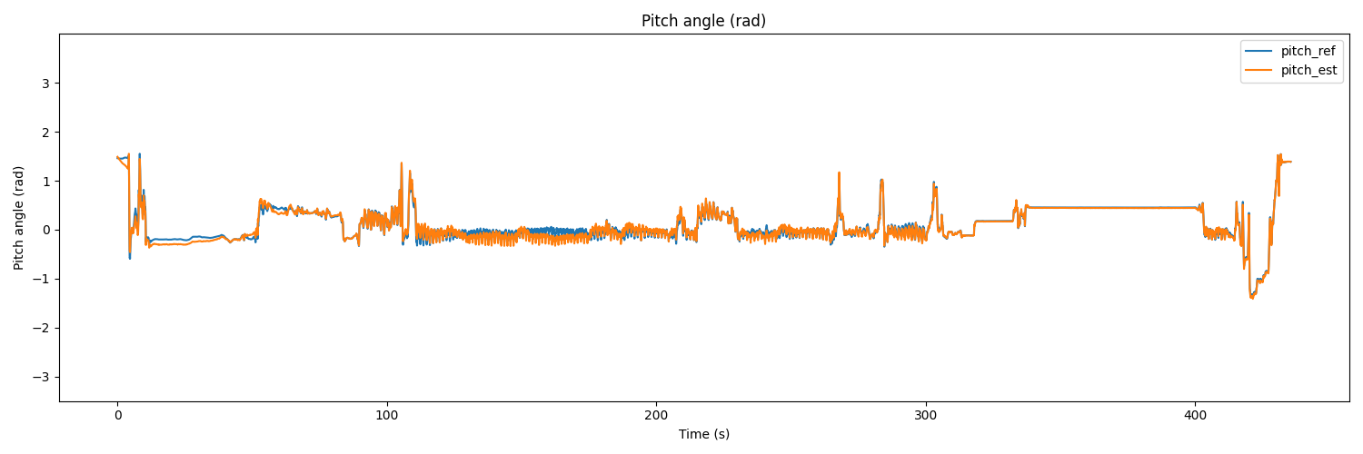
# Pitch
plt.figure(figsize=(15, 5))
plt.plot(t, pitch_ref, label='pitch_ref')
plt.plot(t, pitch_est, label='pitch_est')
plt.title('Pitch angle (rad)')
plt.xlabel('Time (s)')
plt.ylabel('Pitch angle (rad)')
plt.ylim(-3.5, 3.999)
plt.legend(loc='upper right')
plt.show()
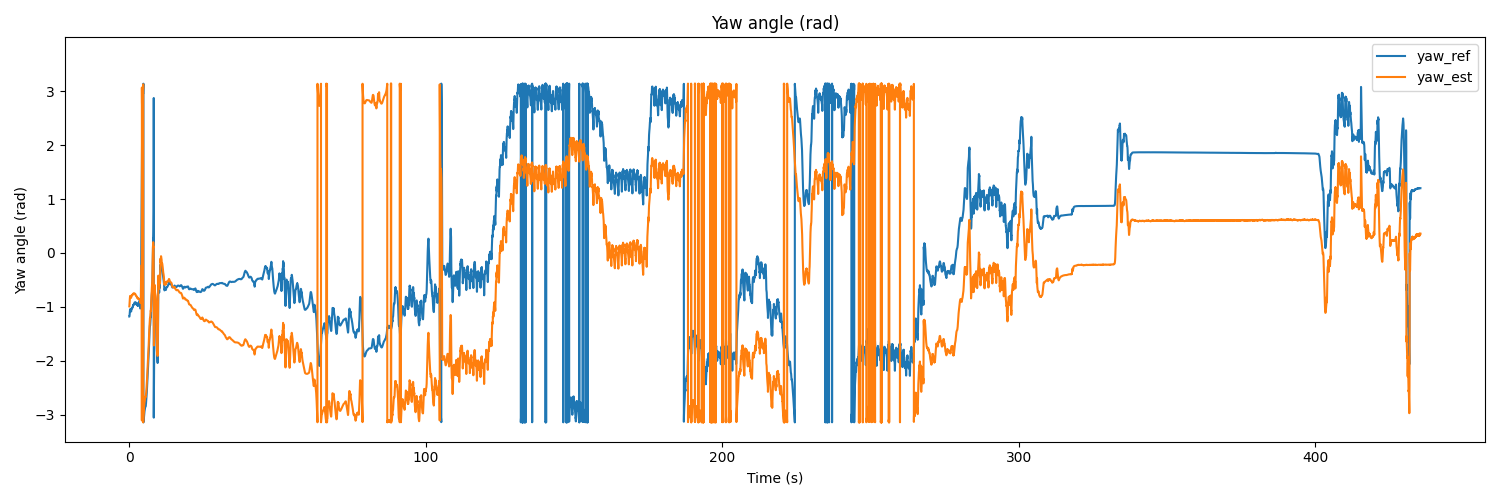
# Yaw
plt.figure(figsize=(15, 5))
plt.plot(t, yaw_ref, label='yaw_ref')
plt.plot(t, yaw_est, label='yaw_est')
plt.title('Yaw angle (rad)')
plt.xlabel('Time (s)')
plt.ylabel('Yaw angle (rad)')
plt.ylim(-3.5, 3.999)
plt.legend(loc='upper right')
plt.show()
The result would be as follows
References
[1] H. Yan, H. Sachini, and F. Yasutaka. “Ronin: Robust neural inertial navigation in the wild: Benchmark, evaluations, and new methods.” arXiv preprint arXiv:1905.12853, 2019. link
Arman Asgharpoor Golroudbari
Machine Learning Engineer
Machine Learning Engineer with 5+ years of experience in LLMs, transformer architectures, computer vision systems, and autonomous robotics.