⇐ Natural Language Processing

Understanding Self-Attention - A Step-by-Step Guide

Self-attention is a fundamental concept in natural language processing (NLP) and deep learning, especially prominent in transformer-based models. In this post, we will delve into the self-attention mechanism, providing a step-by-step guide from scratch.

Self-attention has gained widespread adoption in various models following the publication of the Transformer paper, ‘Attention Is All You Need,’ garnering significant attention in the field.

1. Introduction

Self-attention, also known as scaled dot-product attention, is a fundamental concept in the field of NLP and deep learning. It plays a pivotal role in tasks such as machine translation, text summarization, and sentiment analysis. Self-attention enables models to weigh the importance of different parts of an input sequence when making predictions or capturing dependencies between words.

2. Understanding Attention

Before we dive into self-attention, let’s grasp the broader concept of attention. Imagine reading a long document; your focus naturally shifts from one word to another, depending on the context. Attention mechanisms in deep learning mimic this behavior, allowing models to selectively concentrate on specific elements of the input data while ignoring others.

For instance, in the sentence “The cat sat on the mat,” attention helps you recognize that “mat” is the crucial word for understanding the sentence.

3. Self-Attention Overview

Picture self-attention as the conductor of an orchestra, orchestrating the harmony of information within an input embedding. Its role is to imbue contextual wisdom, allowing the model to discern the significance of individual elements within a sequence and dynamically adjust their influence on the final output. This orchestration proves invaluable in language processing tasks, where the meaning of a word hinges upon its companions in the sentence or document.

The Quartet: Q, K, V, and Self-Attention

At the heart of self-attention are the quartet of Query ($Q$), Key ($K$), Value ($V$), and Self-Attention itself. These components work together in a symphony:

• Query ($Q$): Think of the queries as the elements seeking information. For each word in the input sequence, a query vector is calculated. These queries represent what you want to pay attention to within the sequence.

• Key ($K$): Keys are like signposts. They help identify and locate important elements in the sequence. Like queries, key vectors are computed for each word.

• Value ($V$): Values carry the information. Once again, for each word, a value vector is computed. These vectors hold the content that we want to consider when determining the importance of words in the sequence.

1. Query, Key, and Value Calculation: For each word in the input sequence, we calculate query ($Q$), key ($K$), and value ($V$) vectors. These vectors are the foundation upon which the attention mechanism operates.

2. Attention Scores: With the quartet prepared, attention scores are computed for each pair of words in the sequence. The attention score between a query and a key quantifies their compatibility or relevance.

3. Weighted Aggregation: Finally, the attention scores are used as weights to perform a weighted aggregation of the value vectors. This aggregation results in the self-attention output, representing an enhanced and contextually informed representation of the input sequence.

The Symphony of Self-Attention

Self-attention is not just a mechanism; it’s a symphony of operations that elevate the understanding of sequences in deep learning models. Its adaptability and ability to capture intricate relationships are what make modern NLP models, like transformers, so powerful.

4. Embedding an Input Sentence

In natural language processing (NLP), representing words and sentences in a numerical format is essential for machine learning models to understand and process text. This process is known as “word embedding” or “sentence embedding,” and it forms the foundation for many NLP tasks. In this section, we’ll delve into the concept of word embeddings and demonstrate how to embed a sentence using Python.

Word Embeddings

Word embeddings are numerical representations of words, designed to capture semantic relationships between words. The idea is to map each word to a high-dimensional vector, where similar words are closer in the vector space. One of the most popular word embeddings is Word2Vec, which generates word vectors based on the context in which words appear in a large corpus of text.

Let’s look at an example using the Gensim library to create Word2Vec embeddings:

# Import the Gensim library
from gensim.models import Word2Vec

# Sample sentences for training the Word2Vec model
sentences = [
    ['machine', 'learning', 'is', 'fascinating'],
    ['natural', 'language', 'processing', 'is', 'important'],
    ['word', 'embeddings', 'capture', 'semantic', 'relations'],
]

# Train the Word2Vec model
model = Word2Vec(sentences, vector_size=100, window=5, min_count=1, sg=0)

# Get the word vector for a specific word
vector = model.wv['machine']
print(vector)

[-1.9442164e-03 -5.2675214e-03  9.4471136e-03 -9.2987325e-03
  4.5039477e-03  5.4041781e-03 -1.4092624e-03  9.0070926e-03
  9.8853596e-03 -5.4750429e-03 -6.0210000e-03 -6.7469729e-03
 -7.8948820e-03 -3.0479168e-03 -5.5940272e-03 -8.3446801e-03
  7.8290224e-04  2.9946566e-03  6.4147436e-03 -2.6289499e-03
 -4.4534765e-03  1.2495709e-03  3.9146186e-04  8.1169987e-03
  1.8280029e-04  7.2315861e-03 -8.2645155e-03  8.4335366e-03
 -1.8889094e-03  8.7011540e-03 -7.6168370e-03  1.7963862e-03
  1.0564864e-03  4.6005251e-05 -5.1032533e-03 -9.2476979e-03
 -7.2642174e-03 -7.9511739e-03  1.9137275e-03  4.7846674e-04
 -1.8131376e-03  7.1201660e-03 -2.4756920e-03 -1.3473093e-03
 -8.9005642e-03 -9.9254129e-03  8.9493981e-03 -5.7539381e-03
 -6.3729975e-03  5.1994072e-03  6.6699935e-03 -6.8316413e-03
  9.5975993e-04 -6.0084737e-03  1.6473436e-03 -4.2892788e-03
 -3.4407973e-03  2.1856665e-03  8.6615775e-03  6.7281104e-03
 -9.6770572e-03 -5.6221043e-03  7.8803329e-03  1.9893574e-03
 -4.2560520e-03  5.9881213e-04  9.5209610e-03 -1.1027169e-03
 -9.4246380e-03  1.6084099e-03  6.2323548e-03  6.2823701e-03
  4.0916502e-03 -5.6502391e-03 -3.7069322e-04 -5.5317880e-05
  4.5717955e-03 -8.0415895e-03 -8.0183093e-03  2.6475071e-04
 -8.6082993e-03  5.8201565e-03 -4.1781188e-04  9.9711772e-03
 -5.3439774e-03 -4.8613906e-04  7.7567734e-03 -4.0679323e-03
 -5.0159004e-03  1.5900708e-03  2.6506938e-03 -2.5649595e-03
  6.4475285e-03 -7.6599526e-03  3.3935606e-03  4.8997044e-04
  8.7321829e-03  5.9827138e-03  6.8153618e-03  7.8225443e-03]

In this example, we first import the Gensim library, which provides tools for creating and using word embeddings. We then define a list of sentences to train our Word2Vec model. The vector_size parameter specifies the dimensionality of the word vectors, window controls the context window size, min_count sets the minimum frequency for words to be considered, and sg (skip-gram) indicates the training algorithm.

After training, you can access the word vectors using model.wv['word'], where ‘word’ is the word you want to obtain a vector for.

Sentence Embeddings

While word embeddings represent individual words, sentence embeddings capture the overall meaning of a sentence. One popular method for obtaining sentence embeddings is by averaging the word vectors in the sentence:

import numpy as np

# Sample sentence and its word embeddings
sentence = ['machine', 'learning', 'is', 'fascinating']
word_vectors = [model.wv[word] for word in sentence]

# Calculate the sentence embedding by averaging word vectors
sentence_embedding = np.mean(word_vectors, axis=0)
print(sentence_embedding)

In this code, we take a sample sentence and obtain the word embeddings for each word in the sentence using the Word2Vec model we trained earlier. We then calculate the sentence embedding by averaging the word vectors. This gives us a numerical representation of the entire sentence.

Sentence embeddings are useful for various NLP tasks, including text classification, sentiment analysis, and information retrieval.

Pre-trained Embeddings

In many NLP projects, it’s common to use pre-trained word embeddings or sentence embeddings. These embeddings are generated from large corpora and capture general language patterns. Popular pre-trained models include Word2Vec, GloVe, and BERT.

Here’s how you can load pre-trained word embeddings using Gensim with the GloVe model:

from gensim.models import KeyedVectors

# Load pre-trained GloVe embeddings
glove_model = KeyedVectors.load_word2vec_format('glove.6B.100d.txt', binary=False)

# Get the word vector for a specific word
vector = glove_model['machine']
print(vector)

In this example, we load pre-trained GloVe embeddings from a file (‘glove.6B.100d.txt’ in this case) and access word vectors using glove_model['word'].

In summary, word and sentence embeddings play a pivotal role in NLP tasks, allowing us to represent text data numerically. Whether you create your own embeddings or use pre-trained models, embeddings are a fundamental component in building powerful NLP models.

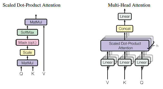
4. The Mathematics of Self-Attention

Mathematically, self-attention can be expressed as:

Given an input sequence of vectors $X = [x_1, x_2, …, x_n]$, where $x_i$ is a vector representing the i-th element in the sequence, we compute the self-attention output $Y$ as follows:

$$ Y = \text{softmax}\left(\frac{QK^T}{\sqrt{d_k}}\right)V $$

• $Q$ (Query), $K$ (Key), and $V$ (Value) are learned linear transformations of the input sequence $X$, parameterized by weight matrices $W_Q$, $W_K$, and $W_V$, respectively.
• $d_k$ is the dimension of the key vectors, often chosen to match the dimension of the query and value vectors.
• $\text{softmax}$ is the softmax function applied along the rows of the matrix.
• $QK^T$ is the matrix of dot products between query and key vectors.
• The resulting matrix is used to weight the value vectors.

Now, let’s break down each step with a detailed example.

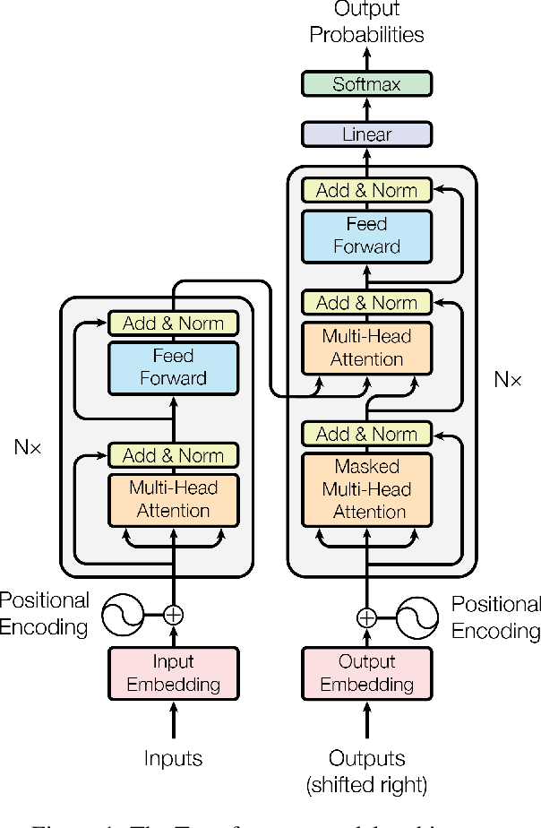
5. Self-Attention in Transformers

Transformers, the backbone of modern NLP models, prominently feature self-attention. In a transformer architecture, self-attention is applied in parallel multiple times, followed by feedforward layers. Here’s a detailed view of how it operates in a transformer:

• Query, Key, and Value: Each input vector $x_i$ is linearly transformed into three vectors: query ($q_i$), key ($k_i$), and value ($v_i$). These transformations are achieved through learned weight matrices $W_Q$, $W_K$, and $W_V$. These vectors are used to compute attention scores.

• Attention Scores: The attention score between a query vector $q_i$ and a key vector $k_j$ is computed as their dot product:

$$ \text{Attention}(q_i, k_j) = q_i \cdot k_j $$

• Scaled Attention: To stabilize training and control gradient magnitudes, the dot products are scaled down by a factor of $\sqrt{d_k}$, where $d_k$ is the dimension of the key vectors:

$$ \text{Scaled Attention}(q_i, k_j) = \frac{q_i \cdot k_j}{\sqrt{d_k}} $$

• Attention Weights: The scaled attention scores are passed through a softmax function to obtain attention weights that sum to 1:

$$ \text{Attention Weight}(q_i, k_j) = \text{softmax}(\text{Scaled Attention}(q_i, k_j)) $$

• Weighted Sum: Finally, the attention weights are used to compute a weighted sum of the value vectors:

$$ \text{Self-Attention}(X) = \sum_j \text{Attention Weight}(q_i, k_j) \cdot v_j $$

Now, let’s work through a step-by-step example to illustrate how self-attention operates.

6. Step-by-Step Example

Let’s consider a simple input sequence $X$ with three vectors, each of dimension 4:

X = [
  [1, 0, 0, 1],
  [0, 2, 2, 0],
  [1, 1, 0, 0]
]

We’ll perform self-attention on this sequence.

Step 1: Query, Key, and Value Transformation

We initiate the process by linearly transforming each vector in $X$ into query ($Q$), key ($K$), and value ($V$) vectors using learned weight matrices $W_Q$, $W_K$, and $W_V$. For this example, let’s assume the weight matrices are as follows:

W_Q = [
  [0.5, 0.2, 0.1, 0.3],
  [0.1, 0.3, 0.2, 0.5],
  [0.3, 0.1, 0.5, 0.2]
]

W_K = [
  [0.4, 0.1, 0.3, 0.2],
  [0.

2, 0.4, 0.1, 0.3],
  [0.3, 0.2, 0.4, 0.1]
]

W_V = [
  [0.2, 0.3, 0.1, 0.4],
  [0.4, 0.2, 0.3, 0.1],
  [0.1, 0.4, 0.2, 0.3]
]

Now, we compute the query, key, and value vectors for each element in $X$:

For the first element $x_1$:

• $q_1 = X[1] \cdot W_Q = [1, 0, 0, 1] \cdot [0.5, 0.2, 0.1, 0.3] = 0.8$
• $k_1 = X[1] \cdot W_K = [1, 0, 0, 1] \cdot [0.4, 0.1, 0.3, 0.2] = 0.6$
• $v_1 = X[1] \cdot W_V = [1, 0, 0, 1] \cdot [0.2, 0.3, 0.1, 0.4] = 0.6$

For the second element $x_2$:

• $q_2 = X[2] \cdot W_Q = [0, 2, 2, 0] \cdot [0.1, 0.3, 0.2, 0.5] = 1.0$
• $k_2 = X[2] \cdot W_K = [0, 2, 2, 0] \cdot [0.2, 0.4, 0.1, 0.3] = 0.6$
• $v_2 = X[2] \cdot W_V = [0, 2, 2, 0] \cdot [0.4, 0.2, 0.3, 0.1] = 0.8$

For the third element $x_3$:

• $q_3 = X[3] \cdot W_Q = [1, 1, 0, 0] \cdot [0.3, 0.1, 0.5, 0.2] = 0.6$
• $k_3 = X[3] \cdot W_K = [1, 1, 0, 0] \cdot [0.3, 0.2, 0.4, 0.1] = 0.5$
• $v_3 = X[3] \cdot W_V = [1, 1, 0, 0] \cdot [0.1, 0.4, 0.2, 0.3] = 0.5$

Step 2: Attention Scores

Now that we have the query ($q_i$) and key ($k_j$) vectors for each element, we calculate the attention scores between all pairs of elements:

• Attention between $x_1$ and $x_1$: $\text{Attention}(q_1, k_1) = 0.8 \cdot 0.6 = 0.48$
• Attention between $x_1$ and $x_2$: $\text{Attention}(q_1, k_2) = 0.8 \cdot 0.6 = 0.48$
• Attention between $x_1$ and $x_3$: $\text{Attention}(q_1, k_3) = 0.8 \cdot 0.5 = 0.40$

Continue this process for all pairs of elements.

Step 3: Scaled Attention

To stabilize the attention scores during training and prevent issues related to gradient vanishing or exploding, the dot products are scaled down by a factor of $\sqrt{d_k}$. For this example, let’s assume $d_k = 4$:

• Scaled Attention between $x_1$ and $x_1$: $\text{Scaled Attention}(q_1, k_1) = \frac{0.48}{\sqrt{4}} = 0.24$
• Scaled Attention between $x_1$ and $x_2$: $\text{Scaled Attention}(q_1, k_2) = \frac{0.48}{\sqrt{4}} = 0.24$
• Scaled Attention between $x_1$ and $x_3$: $\text{Scaled Attention}(q_1, k_3) = \frac{0.40}{\sqrt{4}} = 0.20$

Continue this process for all pairs of elements.

Step 4: Attention Weights

Apply the softmax function to the scaled attention scores to obtain attention weights:

• Attention Weight between $x_1$ and $x_1$: $\text{Attention Weight}(q_1, k_1) = \text{softmax}(0.24) \approx 0.5987$
• Attention Weight between $x_1$ and $x_2$: $\text{Attention Weight}(q_1, k_2) = \text{softmax}(0.24) \approx 0.5987$
• Attention Weight between $x_1$ and $x_3$: $\text{Attention Weight}(q_1, k_3) = \text{softmax}(0.20) \approx 0.5799$

Continue this process for all pairs of elements.

Step 5: Weighted Sum

Finally, we compute the weighted sum of the value vectors using the attention weights:

• Weighted Sum for $x_1$: $\text{Self-Attention}(x_1) = 0.5987 \cdot v_1 + 0.5987 \cdot v_2 + 0.5799 \cdot v_3$

This weighted sum represents the self-attention output for $x_1$. Repeat this process for $x_2$ and $x_3$ to get the self-attention outputs for all elements in the sequence.

7. Multi-Head Attention

In practical applications, self-attention is often extended to multi-head attention. Instead of relying on a single set of learned transformations ($W_Q$, $W_K$, $W_V$), multi-head attention uses multiple sets of transformations, or “heads.” Each head focuses on different aspects or relationships within the input sequence. The outputs of these heads are concatenated and linearly combined to produce the final self-attention output. This mechanism allows models to capture various types of information simultaneously.

8. Positional Encoding

One critical aspect of self-attention is that it doesn’t inherently capture the sequential order of elements in the input sequence, as it computes attention based on content alone. To address this limitation, positional encodings are added to the input embeddings in transformers. These encodings provide the model

with information about the positions of words in the sequence, enabling it to distinguish between words with the same content but different positions.

9. Applications of Self-Attention

Self-attention has found applications beyond NLP and transformers. It has been used in computer vision for tasks like image segmentation, where capturing long-range dependencies is crucial. Additionally, self-attention mechanisms have been adapted for recommendation systems, speech processing, and even reinforcement learning.

10. Conclusion

Self-attention is a cornerstone of modern deep learning, playing a vital role in understanding and processing sequential data effectively. This comprehensive guide has explored the theoretical foundations, mathematical expressions, practical applications, and a detailed step-by-step example of self-attention. By mastering self-attention, you gain insight into the inner workings of state-of-the-art models in NLP and other domains, opening the door to creating more intelligent and context-aware AI systems.