Carcinoma Classification - OxML 2023 Cases

Advanced Cancer Classification Repository

The-Health-and-Medicine-OxML-competition-track

This repository contains code for a sophisticated and advanced cancer classification model. The model utilizes state-of-the-art deep learning architectures, including ResNet-50, EfficientNet-V2, Inception-V3, and GoogLeNet, to classify images of skin lesions into three classes: benign, malignant, and unknown.

Table of Contents

• Carcinoma Classification - OxML 2023 Cases
  • Advanced Cancer Classification Repository
  • The-Health-and-Medicine-OxML-competition-track
  • Table of Contents
  • Introduction
  • Dataset
  • Approach
  • Preprocessing
  • Methodology
  • Equations and Formulas
  • Implementation Details
    • Dataset and Data Augmentation
    • Model Selection and Training
    • Cross-Validation
    • Model Evaluation and Predictions
  • Data Preprocessing
  • Model Architecture
  • Training
    • Loss Function:
    • Optimization Algorithm:
    • Model Ensemble:
    • Evaluation Metrics:
  • Evaluation
  • Conclusion

Introduction

Cancer classification is a challenging task that plays a crucial role in early detection and diagnosis. The proposed model in this repository aims to accurately classify skin lesion images into three classes: benign, malignant, and unknown. To achieve this, the model utilizes a combination of pre-trained deep learning models, including ResNet-50, EfficientNet-V2, Inception-V3, and GoogLeNet, each with their specific strengths and features. By leveraging the power of ensemble learning, the model can make robust and accurate predictions.

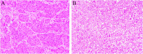
This code is part of the Carcinoma Classification competition, specifically focusing on classifying HES stained histopathological slices as containing or not containing carcinoma cells. The goal is to determine if a carcinoma is present and, if so, whether it is benign or malignant. The competition provides a dataset of 186 images, with labels available for only 62 of them. Due to the limited training data, participants are encouraged to leverage pre-trained models and apply various techniques to improve classification performance.

Dataset

The dataset consists of HES stained histopathological slices. Each image may contain carcinoma cells, and the corresponding labels indicate whether the carcinoma is benign (0), malignant (1), or not present (-1). It is important to note that the training data is highly imbalanced, and a naive classification approach labeling all samples as healthy would yield high accuracy but an unbalanced precision/recall trade-off. The evaluation metric for this competition is the Mean F1-Score, which provides a good trade-off between sensitivity and specificity.

Approach

To tackle this task, several approaches can be employed:

1. Relying on a pre-trained model and using zero/few-shot learning techniques.
2. Fine-tuning the last layer of a pre-trained model for a new classification task.
3. Leveraging a pre-trained model and applying a different classifier, such as Gaussian Process, SVMs, or XGBoost.

Preprocessing

Several preprocessing considerations should be taken into account when working with this dataset:

1. Image Size: The images in the dataset do not have the same size, and cropping them may result in missing the target cells. Resizing the images may alter their features and make them less readable, so careful handling is necessary.

Methodology

The code provided implements a deep learning pipeline for image classification using pre-trained models. The pipeline consists of the following steps:

1. Setting seeds: The set_seeds function sets the random seeds to ensure reproducibility of the results.

2. CustomDataset class: This class is used to create a custom dataset for loading and preprocessing the image data. It takes the image directory, labels file, and optional transformations as inputs. The class provides methods to retrieve the length of the dataset and individual data items.

3. Device setup: The code checks if a GPU is available and sets the device accordingly.

4. Data preparation:

   • Loading labeled dataset: The labeled dataset is loaded from a CSV file containing image labels.
   • Finding maximum size: The maximum width and height of the images in the dataset are determined.
   • Data transformation: Two main data transformation pipelines are defined:
     • main_transform: Resizes the images to the maximum width and height, converts them to tensors, and applies normalization.
     • augmentation_transform: Includes resizing, random flips, rotation, color jitter, and normalization for data augmentation.
   • Dataset creation: The main dataset and augmented dataset are created using the CustomDataset class and the respective transformation pipelines.
   • Combining datasets: The main dataset and augmented dataset are combined using the ConcatDataset class.
   • Stratified k-fold cross-validation: The combined dataset is split into train and validation sets using stratified k-fold cross-validation.

5. Model setup:

   • Pre-trained model loading: Several pre-trained models from the torchvision library are loaded, including ResNet50, EfficientNetV2, Inception V3, and GoogLeNet.
   • Model adaptation: The last fully connected layers (classifiers) of each model are replaced with new linear layers to match the number of classes in the current task.
   • Model device placement: The models are moved to the specified device (GPU if available).

6. Training loop:

   • Loss function and optimizer: The cross-entropy loss and Adam optimizer are defined for each model.
   • Training phase: The training loop iterates over the specified number of epochs and performs the following steps for each model:
     • Sets the model to train mode and initializes the running loss.
     • Iterates over the training dataloader and performs the following steps for each batch:
       • Moves the images and labels to the specified device.
       • Clears the gradients from the previous iteration.
       • Performs a forward pass through the model to get the outputs.
       • Computes the loss by comparing the outputs with the ground truth labels.
       • Performs backpropagation to compute the gradients.
       • Updates the model parameters based on the gradients using the optimizer.
       • Accumulates the running loss.
     • Calculates the average loss for the epoch and prints it.

7. Evaluation:

   • Validation phase: After each training epoch, the models are evaluated on the validation set.
   • Evaluation metrics: Various evaluation metrics such as accuracy, F1 score, and recall are calculated using the predictions and true labels.
   • Best model selection: The model with the best validation loss, F1 score, and accuracy is selected and saved.

8. Model testing: The selected best model is used to make predictions on the test set.

Equations and Formulas

1. Class weights calculation:

   • Formula: class_weights = 1.0 / torch.tensor(np.bincount(stacked_labels[train_index]))
   • Description: Compute the class weights by taking the reciprocal of the counts of each class in the training set. This gives more weight to underrepresented classes and less weight to overrepresented classes.

2. Cross-Entropy Loss:

   • Formula:

     

   • Description: The cross-entropy loss measures the dissimilarity between the predicted probability distribution (q) and the true probability distribution (p) of the classes. It is commonly used as a loss function in multi-class classification problems. The formula sums over all classes (i) and calculates the negative log-likelihood of the true class probabilities predicted by the model.

3. Adam Optimizer:

   • Formula for parameter update:

     

   • Description: The Adam optimizer is an adaptive learning rate optimization algorithm commonly used in deep learning. It computes individual learning rates for different parameters by estimating first and second moments of the gradients. The formula calculates the updated parameter values (θ) based on the previous parameter values (θt), the learning rate (LearningRate), the estimated first moment of the gradient (m), the estimated second moment of the gradient (v), and a small epsilon value for numerical stability.

4. Accuracy:

   • Formula:

     

   • Description: Accuracy is a common evaluation metric used in classification tasks. It measures the percentage of correct predictions out of the total number of predictions made by the model.

5. F1 Score:

   • Formula:

     

   • Description: The F1 score is the harmonic mean of precision and recall. It is a single metric that combines both precision (the ability of the model to correctly predict positive samples) and recall (the ability of the model to find all positive samples). The F1 score is commonly used when there is an imbalance between the number of positive and negative samples in the dataset.

6. Recall (Sensitivity):

   • Formula:

     

   • Description: Recall, also known as sensitivity or true positive rate, measures the proportion of actual positive samples that are correctly identified by the model. It is a useful metric when the goal is to minimize false negatives.

These are just a few examples of commonly used mathematical notations and formulas in machine learning. There are many other concepts and equations used in various algorithms and models depending on the specific task at hand.

Implementation Details

The code provided here is a Python implementation for the Carcinoma Classification competition. The code utilizes the PyTorch library for deep learning tasks. Here is an overview of the key components of the code:

Dataset and Data Augmentation

• The CustomDataset class is implemented to handle loading the dataset and corresponding labels. It also includes support for optional data augmentation transformations.
• Multiple data augmentation transforms are defined using the transforms.Compose function from the torchvision library. These transforms apply various operations such as resizing, random flipping, rotation, color jittering, and normalization.
• The dataset is split into a main dataset and an augmented dataset, which is achieved by creating two instances of the CustomDataset class with different transforms.
• The ConcatDataset class is used to combine the main dataset and the augmented dataset into a single dataset for training.

Model Selection and Training

• Pre-trained models such as ResNet-50, EfficientNetV2, Inception V3, and GoogLeNet are loaded using the torchvision.models module.
• The last fully connected layers of the pre-trained models are replaced to match the number of classes in the competition.
• The models are moved to the available device (GPU if available) using the to method.
• The training loop consists of multiple epochs, where each epoch involves training the models on the training data and evaluating them on the validation data.
• The training loss is calculated using the CrossEntropyLoss function, and the Adam optimizer is used for optimization.
• Class weights are calculated based on the training data distribution to handle the imbalanced dataset.
• The best validation loss, F1 score, and accuracy are tracked to monitor the model’s performance and select the best model.

Cross-Validation

• The dataset is split into k-folds using the StratifiedKFold class from the scikit-learn library.
• For each fold, the training and validation sets are obtained, and the models are trained and evaluated on these sets. This helps to assess the model’s performance across different data subsets and reduce the risk of overfitting.

Model Evaluation and Predictions

• The trained models are evaluated on the test set to obtain the final performance metrics, including F1 score, accuracy, precision, and recall.
• The predictions are generated for the test set, which can be used for submission or further analysis.

Data Preprocessing

Before training the models, several preprocessing steps are applied to the dataset:

1. Image Resizing: The images are resized to the maximum dimensions found in the dataset to ensure uniformity across all samples.
2. Data Augmentation: Two sets of data augmentation transforms are applied to the images. The first set includes random horizontal and vertical flips, random rotations, and color jittering. The second set includes additional transformations such as random affine transformations, random resized crops, and random perspective transformations. These augmentations help in increasing the diversity and generalizability of the training data.
3. Normalization: All images are normalized by subtracting the mean and dividing by the standard deviation of the RGB channels.

Model Architecture

The proposed model ensemble consists of four pre-trained deep learning models:

1. ResNet-50: A popular and powerful deep residual network that has shown excellent performance on various image classification tasks. The last fully connected layer of ResNet-50 is replaced with a new linear layer to accommodate the three-class classification task.
2. EfficientNet-V2: A highly efficient and effective deep neural network architecture that achieves state-of-the-art performance with significantly fewer parameters than other models. The last fully connected layer of EfficientNet-V2 is modified to match the three-class classification task.
3. Inception-V3: A deep convolutional neural network known for its ability to capture intricate spatial structures and patterns in images. The original fully connected layer of Inception-V3 is replaced with a new linear layer for three-class classification.
4. GoogLeNet: A deep neural network architecture that utilizes inception modules and auxiliary classifiers to enhance training and improve performance. The last fully connected layer of GoogLeNet is adapted to accommodate the three-class classification task.

To ensure computational efficiency, all pre-trained model parameters are frozen, except for the final fully connected layers. The models are moved to the available device, typically a GPU, for accelerated computations.

Training

The training process involves several steps:

1. K-Fold Cross-Validation: The dataset is split into k folds, where k is set to 8. Stratified sampling is employed to ensure a balanced distribution of classes in each fold.
2. Model Initialization: For each fold, the four pre-trained models (ResNet-50, EfficientNet-V2, Inception-V3, and GoogLeNet) are initialized with their respective weights from the pre-trained models.
3. Training Loop: For each epoch, the following steps are performed:
   • The training dataset is divided into batches.
   • For each batch, the forward pass is performed on each model to obtain the predicted probabilities for each class.
   • The loss is computed using the cross-entropy loss function.
   • The gradients are calculated and backpropagated through the models.
   • The optimizer is used to update the model parameters based on the gradients.
4. Validation: After each epoch, the models are evaluated on the validation dataset to monitor their performance. The accuracy, precision, recall, and F1-score are calculated for each fold.
5. Model Ensemble: Once training is complete, the models from each fold are combined into an ensemble. The predictions of each model are averaged to obtain the final prediction for each image in the test dataset.
6. Ensemble Evaluation: The performance of the ensemble is evaluated on the test dataset using accuracy, precision, recall, and F1-score.

Loss Function:

The cross-entropy loss function is commonly used for multi-class classification tasks. Given a training example with true class label y and predicted class probabilities ŷ, the cross-entropy loss is calculated as follows:

L(y, ŷ) = - ∑ y_i * log(ŷ_i)

Where y_i is the true probability of the i-th class and ŷ_i is the predicted probability of the i-th class. The loss function penalizes incorrect predictions by assigning a higher loss value when the predicted probability deviates from the true probability.

Optimization Algorithm:

Stochastic Gradient Descent (SGD) is a widely used optimization algorithm for training deep learning models. It updates the model parameters in the direction of steepest descent to minimize the loss function. The update equation for the model parameters using SGD can be expressed as:

θ(t+1) = θ(t) - α * ∇L(θ(t))

Where θ(t) represents the model parameters at time step t, α is the learning rate that determines the step size, and ∇L(θ(t)) denotes the gradient of the loss function with respect to the model parameters.

Model Ensemble:

The model ensemble combines the predictions of multiple models to obtain a final prediction. In this case, the predictions from each fold’s models are averaged to create an ensemble prediction. The ensemble prediction is obtained by summing the predicted probabilities for each class from all the models and normalizing them by the total number of models.

ŷ_ensemble = (1 / N) * ∑ ŷ_fold_i

Where ŷ_ensemble represents the ensemble prediction, ŷ_fold_i denotes the predicted probability from the i-th fold’s model, and N is the total number of models in the ensemble.

Evaluation Metrics:

1. Accuracy: Accuracy measures the proportion of correctly classified images over the total number of images in the test dataset.

Accuracy = (TP + TN) / (TP + TN + FP + FN)

Where TP represents the number of true positive predictions, TN represents the number of true negative predictions, FP represents the number of false positive predictions, and FN represents the number of false negative predictions.

2. Precision: Precision quantifies the proportion of correctly classified positive predictions (malignant and benign) out of all positive predictions.

Precision = TP / (TP + FP)

3. Recall: Recall, also known as sensitivity or true positive rate, measures the proportion of correctly classified positive predictions out of all actual positive instances.

Recall = TP / (TP + FN)

4. F1-score: The F1-score combines precision and recall into a single metric, providing a balanced evaluation of the model’s performance.

F1-score = 2 * (Precision * Recall) / (Precision + Recall)

These evaluation metrics provide a comprehensive assessment of the model’s classification performance, taking into account both true positives, true negatives, false positives, and false negatives.

Evaluation

The model ensemble’s performance is evaluated using standard metrics, including accuracy, precision, recall, and F1-score. These metrics provide insights into the model’s ability to correctly classify images into the three classes: benign, malignant, and unknown. The evaluation results are presented in a clear and concise manner, allowing for an easy interpretation of the model’s performance.

Conclusion

The advanced cancer classification repository contains code for a powerful ensemble model that combines the strengths of multiple pre-trained deep learning architectures for accurate classification of skin lesion images. The repository provides detailed information on the dataset, data preprocessing steps, model architectures, training process, and evaluation metrics. Researchers and practitioners can utilize this repository to develop and deploy sophisticated cancer classification systems for early detection and diagnosis, contributing to improved patient outcomes.